Fama-French Portfolio Sorts#
The way to become rich is to put all your eggs in one basket and then watch that basket - Andrew Carnegie
The Fama-French portfolio sorting methodology is widely used in empirical asset pricing research, particularly in understanding the cross-section of stock returns. By classifying stocks based on fundamental characteristics such as book-to-market ratio and firm size, this approach provides insights into the risk and return dynamics of different investment strategies. This notebook also includes linear regression analysis to assess factor exposures, tests for the value and small-firm effects, and a structural break analysis using the Chow test.
import numpy as np
import scipy
from scipy.stats import skew, kurtosis
import pandas as pd
from pandas import DataFrame, Series
import matplotlib.pyplot as plt
import statsmodels.formula.api as smf
from finds.database import SQL, RedisDB
from finds.structured import BusDay, CRSP, CRSPBuffer, Signals, Benchmarks, PSTAT
from finds.utils import plot_date
from finds.backtesting import bivariate_sorts, BackTest
from finds.utils import plot_date, plot_scatter, plot_hist
from tqdm import tqdm
from secret import credentials, CRSP_DATE
VERBOSE = 0
# %matplotlib qt
sql = SQL(**credentials['sql'], verbose=VERBOSE)
user = SQL(**credentials['user'], verbose=VERBOSE)
rdb = RedisDB(**credentials['redis'])
bd = BusDay(sql, verbose=VERBOSE)
crsp = CRSP(sql, bd, rdb=rdb, verbose=VERBOSE)
pstat = PSTAT(sql, bd, verbose=VERBOSE)
signals = Signals(user, verbose=VERBOSE)
bench = Benchmarks(sql, bd, verbose=VERBOSE)
backtest = BackTest(user, bench, rf='RF', max_date=CRSP_DATE, verbose=VERBOSE)
LAST_DATE = bd.endmo(CRSP_DATE, -1)  # last monthly rebalance date
Stock fundementals data#
Compustat#
Compustat is a database containing financial statements and market data for both active and inactive U.S. and international companies. It is commonly used in academic and industry research.
To compute book-to-price ratios from financial statements, we:
Extract balance sheet items from the Compustat Annual dataset.
Construct the High Minus Low (HML) factor by calculating book equity as shareholders’ equity plus investment tax credits, minus preferred stock, divided by the market capitalization at the end of December.
Apply a six-month reporting lag and require at least two years of history in Compustat.
Exclude deferred taxes and investment tax credits from book equity for fiscal years ending in 1993 or later, following FASB 109, which improved the accounting treatment for deferred income taxes.
label = 'hml'
lag = 6               # number of months to lag fundamental data
# retrieve data fields from compustat, linked by permno
df = pstat.get_linked(dataset = 'annual',
                      date_field = 'datadate',
                      fields = ['seq', 'pstk', 'pstkrv', 'pstkl', 'txditc'],
                      where = ("indfmt = 'INDL'"
                               "  AND datafmt = 'STD'"
                               "  AND curcd = 'USD' "
                               "  AND popsrc = 'D'"
                               "  AND consol = 'C'"
                               "  AND seq > 0 "))
# subtract preferred stock
df[label] = np.where(df['pstkrv'].isna(), df['pstkl'], df['pstkrv'])
df[label] = np.where(df[label].isna(), df['pstk'], df[label])
df[label] = np.where(df[label].isna(), 0, df[label])
# do not add back deferred investment tax credit for fiscal years in 1993 or later
df[label] = (df['seq'] - df[label]
             + df['txditc'].fillna(0).where(df['datadate'] // 10000 <= 1993, 0))
df.dropna(subset = [label], inplace=True)
df = df[df[label] > 0][['permno', 'gvkey', 'datadate', label]]
# count years in Compustat
df = df.sort_values(by=['gvkey','datadate'])
df['count'] = df.groupby(['gvkey']).cumcount()
# construct b/m ratio
df['rebaldate'] = 0
for datadate in tqdm(sorted(df['datadate'].unique())):
    f = df['datadate'].eq(datadate)
    rebaldate = bd.endmo(datadate, abs(lag)) # 6 month lag
    capdate = bd.endyr(datadate)   # Dec mktcap
    if rebaldate >= CRSP_DATE or capdate >= CRSP_DATE:
        continue
    df.loc[f, 'rebaldate'] = rebaldate
    df.loc[f, 'cap'] = crsp.get_cap(capdate, use_permco=True)\
                           .reindex(df.loc[f, 'permno'])\
                           .values
df[label] /= df['cap']
df = df[df[label].gt(0) & df['count'].gt(1)]  # 2+ years in Compustat
signals.write(df, label)
100%|██████████| 758/758 [00:02<00:00, 317.69it/s]
227642
Bivariate sorts#
Independent bivariate sorts categorize stocks based on two characteristics: book-to-market ratio and market capitalization. Portfolios are formed at the end of each June and represent the intersections of:
Two groups sorted by size (market equity, ME).
Three groups sorted by book-to-market ratio (BE/ME).
The size breakpoint for year t is the median NYSE market equity at the end of June in that year. Stocks within each of the six resulting portfolios are weighted by market capitalization.
The two key factors derived from these sorts are:
HML (High Minus Low): The equal-weighted average return of the two value portfolios minus the average return of the two growth portfolios.
SMB (Small Minus Big): The equal-weighted average return of the three small-size portfolios minus the average return of the three large-size portfolios.
Causal Analysis
This sorting approach has conceptual parallels with causal analysis techniques. Specifically, propensity score matching is often used in statistical research to mitigate confounding effects when estimating treatment effects. Propensity scores, estimated via logistic regression, allow researchers to:
Stratify subjects into groups based on similar propensity scores.
Match treated and control subjects with comparable propensity scores.
Adjust for imbalances using regression models.
Since firm size directly influences the book-to-market ratio (as its denominator), applying bivariate sorting ensures that value returns are estimated while controlling for the small-firm effect—similar to how propensity score matching controls for confounding variables in observational studies.
HML#
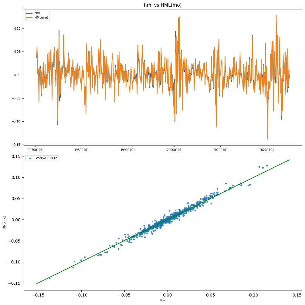
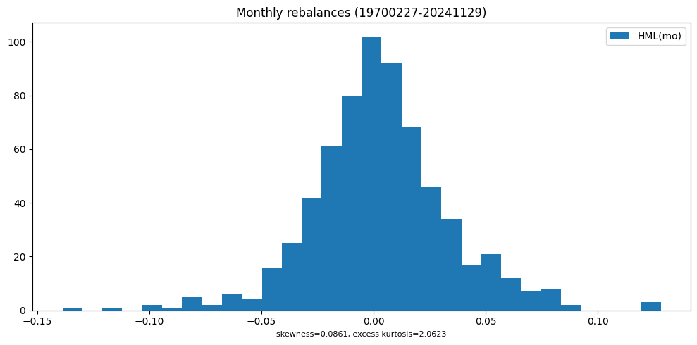
Compute High Minus Low book-to-price monthly returns and compare to Fama-French research factor
label, benchname = 'hml', 'HML(mo)'
rebalend = LAST_DATE
rebalbeg = 19700101
# preload monthly dataset into memory
monthly = CRSPBuffer(stocks=crsp, dataset='monthly',
                     fields=['ret', 'retx', 'prc'],
                     beg=19251201, end=CRSP_DATE)
hml, smb = bivariate_sorts(stocks=monthly,
                           label=label,
                           signals=signals,
                           rebalbeg=rebalbeg,
                           rebalend=rebalend,
                           window=12,
                           months=[6])
Helpers to show histograms and comparisons of portfolio returns
def plot_ff(y, label):
    """helper to scatter plot and compare portfolio returns"""
    y = y.rename(columns={'excess': label})
    corr = np.corrcoef(y, rowvar=False)[0,1]
    fig, (ax1, ax2) = plt.subplots(2, 1, clear=True, figsize=(10, 10))
    plot_date(y, ax=ax1, title=" vs ".join(y.columns), fontsize=7)
    plot_scatter(y.iloc[:,0], y.iloc[:,1], ax=ax2, abline=False, fontsize=7)
    plt.legend([f"corr={corr:.4f}"], fontsize=8)
    plt.tight_layout(pad=0.5)
    print(f"<R-squared of {label} vs {benchname}"
          f" ({y.index[0]} - {y.index[-1]}): {corr*corr:.4f}")
def plot_summary(y, label):
    """helper to plot histogram and statistics of portfolio returns"""
    y = y[label]
    kurt = kurtosis(y, bias=True, fisher=True)  # excess kurtosis
    skewness = skew(y, bias=True)
    fig, ax = plt.subplots(1, 1, clear=True, figsize=(10, 5))
    ax.hist(y, bins=30)
    ax.set_title(f"Monthly rebalances ({y.index[0]}-{y.index[-1]})")
    ax.set_xlabel(f"skewness={skewness:.4f}, excess kurtosis={kurt:.4f}",
                  fontsize=8)
    plt.legend([label])
    plt.tight_layout()
# Plot histogram and comparison of HML returns
holdings = hml
result = backtest(monthly, holdings, label)
y = backtest.fit([benchname], rebalbeg, LAST_DATE)
plot_ff(y, label)
plot_summary(y, benchname)
<R-squared of hml vs HML(mo) (19700227 - 20241129): 0.9784


SMB#
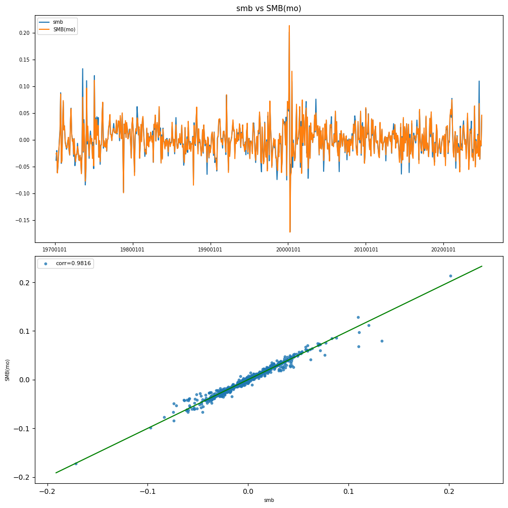
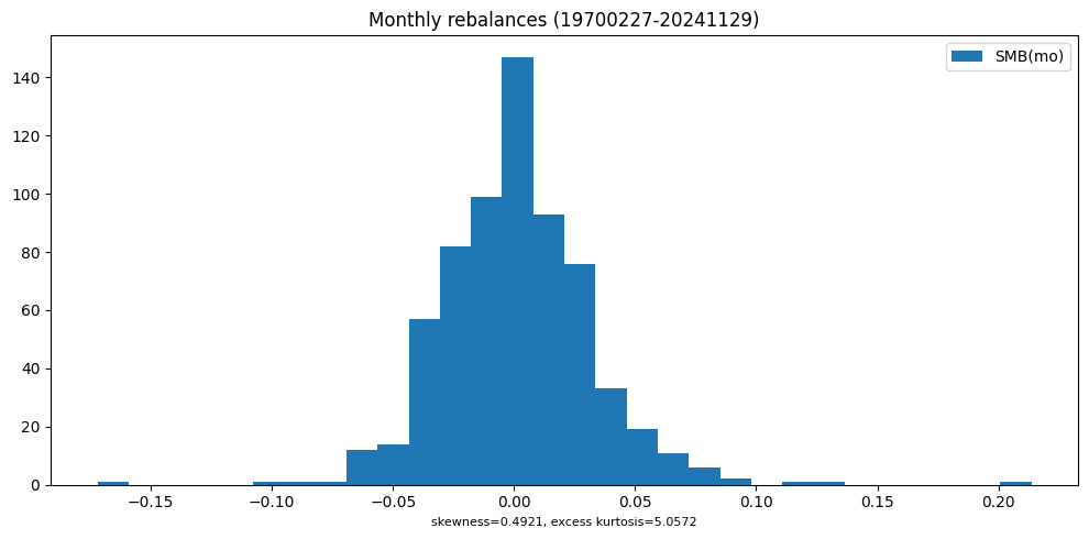
Compare Small-Minus-Big monthly returns and compare to Fama-French research factor
# Plot histogram and comparison of SMB returns
label, benchname = 'smb', 'SMB(mo)'
holdings = smb
result = backtest(monthly, holdings, label)
y = backtest.fit([benchname], rebalbeg, LAST_DATE)
plot_ff(y, label)
plot_summary(y, benchname)
<R-squared of smb vs SMB(mo) (19700227 - 20241129): 0.9636


Linear regression#
Simple Linear Regression
The simple linear regression (SLR) model relates a continuous response (or dependent) variable \(y_i\) with one predictor (or explanatory or independent) variable \(x_i\) and an error term \(\epsilon_i\):
Coefficent estimates of the slope \(b\) and intercept \(a\) are chosen to minimize the residual sum of squares:
Key concepts:
Residuals are the difference between the observed response values and the response values predicted by the model, \(e_i = y_i - \hat{y}_i\).
Residual sum of squares (RSS) over all observations is \(RSS = e^2_1 + e^2_2 + ... + e^2_n\) or equivalently \(RSS = \sum_{i=1}^n (y_i - \hat{y}_i)^2\).
Mean square error (MSE) is an estimate of the variance of the residuals \(s^2 = \hat{\sigma}^2 = \frac{1}{n-2} \sum_{i=1}^n (y_i - \hat{y}_i)^2\).
Residual standard error (RSE) or residual standard deviation is the estimate of the (square root of the) variance of the residuals. Standard error tells us the average amount that the estimate differs from the actual value. The residual standard error is the estimate of the (square root of the) variance of the residuals \(\hat{s} \equiv RSE = \sqrt{RSS/(n - 2)}\).
Hypothesis testing and confidence intervals
The estimators of the coefficients follow a normal distribution in large samples. Therefore, tests of a hypothesis about a regression parameter are implemented using a t-test. The standard errors associated with linear regression coefficient and mean response estimates are:
Slope: \(se(\hat{b}) = \sqrt{\dfrac{s^{2}}{\sum_{i=1}^{n}(x_{i} - \overline{x})^{2}}}\)
Intercept: \(se(\hat{a}) = \sqrt{s^{2}[\dfrac{1}{n} + \dfrac{\overline{x}^{2}}{\sum_{i=1}^{n}(x_{i} - \overline{x})^{2}}]}\)
Mean response: \(se(\hat{y}) = \sqrt{s^2 [\dfrac{1}{n} + \dfrac{(x - \bar{x})^2}{\sum_{i=1}^{n}(x_i - \bar{x})^2}]}\)
Confidence intervals can be computed from standard errors. A 95% confidence interval is defined as a range of values such that with 95% probability, the range will contain the true unknown value of the parameter. The confidence interval for coefficient estimates is:\ \(b_j \pm t_{n - (k + 1), 1 - \frac{\alpha}{2}}\ se(b_j)\), where \(k\), the number of regressors, equals 1 for SLR.
Prediction interval for a new response is \(se(\hat{y}_{n+1}) = \sqrt{s^2 (1 + \dfrac{1}{n} + \dfrac{(x - \bar{x})^2}{\sum_{i=1}^{n}(x_i - \bar{x})^2})}\)
Multiple Linear Regression
With multiple regressors, the linear model \(y = b_0 + b_1 x_1 + ... + b_k x_k + \epsilon\) has coefficient estimates: $\(\hat{b} = (X^T X)^{-1} X^T y\)$
The coefficient \(b_{j}\) quantifies the association between the \(j\) ‘th predictor and the response. It is the average effect on Y of a one unit increase in \(X_j\), holding all other predictors fixed.
Additional concepts:
Sum of squares total (SST) measures the total variance in the response Y, and can be thought of as the amount of variability inherent in the response before the regression is performed. \(\mathrm{SST} = \sum_{i=1}^n (y_i - \overline{y})^2\) measures the total variance in the response Y.
Sum of squares regression (SSR) measures the total amount variance captured by the regression model: \(\mathrm{SSR} = \sum{i=1}^n (\hat{y}_i - \overline{y})^2\)
Sum of squares error (SSE) measures the total variance of the response not explained by the regression model. In the linear regression context, we may intepret total deviation to equal the deviation not explained by the explanatory variables plus deviation explained by the explanatory variables: \((y_i - \overline{y}) = (y_i - \hat{y}_i) + (\hat{y}_i - \overline{y}_i)\).
Squaring each side and summing over all observations yields for the total sum of squared deviations \(SST = \sum_{i=1}^n (y_i - \hat{y}_i)^2 + \sum_{i=1}^n (\hat{y}_i - \overline{y}_i)^2 = SSE + SSR\), where the sum of the cross-product terms turns out to be zero.\(R^2\) statistic or coefficient of determination measures the proportion of variability in Y that can be explained using X. It is also identical to the squared correlation between X and Y. An \(R^2\) statistic that is close to 1 indicates that a large proportion of the variability in the response has been explained by the regression. A number near 0 indicates that the regression did not explain much of the variability in the response. The \(R^2\) statistic provides a relative measure of the quality of a linear regression fit \(R^2 = 1 - \frac{\mathrm{RSS}}{\mathrm{SST}}\), and always takes on a value between 0 and 1, and is independent of the scale. \(R^2\) is identical to the squared correlation between \(X\) and \(Y\).
Adjusted \(R^2\): The usual \(R^2\) always increases (since residual sum of squares RSS always decreases) as more variables are added. The intuition behind the adjusted \(R^2\) is that once all of the correct variables have been included in the model, adding noise variables will lead to a decrease in the statistic. In theory, the model with the largest adjusted \(R^2\) will have only correct variables and no noise variables.
Partial correlation coefficients, which measure the correlation between \(y\) and the \(j\) ‘th explanatory variable \(x_j\) controlling for other explanatory variables, can also be obtained by running only one regression: $\(r(y, x_j | x_1,x_2,...,x_{j-1},x_{j+1},...,x_k) = \frac{t(b_j)}{\sqrt{t(b_j)^2 + n - (k+1)}}\)\( where \)t(b_j)\( is the t-ratio for \)b_j\( from a regression of \)y\( on \)x_1,…,x_k\( (including the variable \)x_j$).
t-statistic or t-ratio: \(t(b_j) = \dfrac{b_j}{se(b_j)}\) can be interpreted to be the number of standard errors that \(b_j\) is away from zero. In a t-test, the null hypothesis (\(H_0: \beta_j = 0\)) is rejected in favor of the alternative if the absolute value of the t-ratio \(|t(b_j)|\) exceeds a t-value, denoted \(t_{n - (k + 1), 1 - \frac{\alpha}{2}}\), equal to the \((1 - \frac{\alpha}{2})\) ‘th percentile from the t-distribution using \(df = n - ( k + 1)\) degrees of freedom.
*Hypothesis tests
The t-test is not directly applicable when testing hypotheses that involve more than one parameter, because the parameter estimators can be correlated. Instead, a common alternative called the F-test compares the fit of the model (measured using the RSS) when the null hypothesis is true relative to the fit of the model without the restriction on the parameters assumed by the null. To test whether all regression slope coefficients are zero \(H_0: b_1 = ... = b_p = 0\), versus the alternative \(H_a :\) at least one \(b_j\) is non-zero, compute the statistic. which has a \(F(p, n-p-1)\) distribution:
Partial F-test: Sometimes, we want to test that a particular subset of \(q\) of the coefficients are zero. In this case we fit a second model that uses all the variables except those last \(q\), then compute residual sum of squares for that model and the appropriate F-statistic, which has a \(F(p-q, n-p-1)\) distribution:
Value effect#
The value effect refers to the observed tendency of value stocks (low price-to-book ratios) to outperform growth stocks (high price-to-book ratios) over time. This phenomenon supports value investing, a strategy linked to Benjamin Graham and David Dodd, which focuses on identifying undervalued stocks based on fundamental analysis.
# Linear regression on Mkt-Rf and intercept
x = ["HML(mo)", "Mkt-RF(mo)"]
formula = f'Q("{x[0]}") ~ ' + " + ".join(f'Q("{v}")' for v in x[1:])
data = bench.get_series(x, field='ret', beg=19620701, end=20991231)
lm = smf.ols(formula, data=data).fit(cov_type='HAC', cov_kwds={'maxlags': 6})
print(f"Period: {data.index[0]}-{data.index[-1]}")
print(lm.summary())
Period: 19620731-20241231
                            OLS Regression Results
==============================================================================
Dep. Variable:           Q("HML(mo)")   R-squared:                       0.041
Model:                            OLS   Adj. R-squared:                  0.040
Method:                 Least Squares   F-statistic:                     8.701
Date:                Sun, 02 Mar 2025   Prob (F-statistic):            0.00328
Time:                        14:45:35   Log-Likelihood:                 1587.2
No. Observations:                 750   AIC:                            -3170.
Df Residuals:                     748   BIC:                            -3161.
Df Model:                           1
Covariance Type:                  HAC
===================================================================================
                      coef    std err          z      P>|z|      [0.025      0.975]
-----------------------------------------------------------------------------------
Intercept           0.0037      0.001      2.615      0.009       0.001       0.006
Q("Mkt-RF(mo)")    -0.1344      0.046     -2.950      0.003      -0.224      -0.045
==============================================================================
Omnibus:                       54.218   Durbin-Watson:                   1.670
Prob(Omnibus):                  0.000   Jarque-Bera (JB):              243.740
Skew:                          -0.030   Prob(JB):                     1.18e-53
Kurtosis:                       5.792   Cond. No.                         22.3
==============================================================================

Notes:
[1] Standard Errors are heteroscedasticity and autocorrelation robust (HAC) using 6 lags and without small sample correction
Small firm effect#
The small firm effect, identified by Rolf Banz in 1981, describes the tendency of small-cap stocks to generate higher risk-adjusted returns than large-cap stocks. This suggests that smaller companies may offer higher expected returns as compensation for their increased risk and lower liquidity.
# Linear regression on Mkt-Rf, HML and intercept
x = ["SMB(mo)", "HML(mo)", "Mkt-RF(mo)"]
formula = f'Q("{x[0]}") ~ ' + " + ".join(f'Q("{v}")' for v in x[1:])
data = bench.get_series(x, field='ret', beg=19620701, end=20991231)
lm = smf.ols(formula, data=data).fit(cov_type='HAC', cov_kwds={'maxlags': 6})
print(f"Period: {data.index[0]}-{data.index[-1]}")
print(lm.summary())
Period: 19620731-20241231
                            OLS Regression Results
==============================================================================
Dep. Variable:           Q("SMB(mo)")   R-squared:                       0.097
Model:                            OLS   Adj. R-squared:                  0.095
Method:                 Least Squares   F-statistic:                     28.64
Date:                Sun, 02 Mar 2025   Prob (F-statistic):           1.03e-12
Time:                        14:45:35   Log-Likelihood:                 1593.2
No. Observations:                 750   AIC:                            -3180.
Df Residuals:                     747   BIC:                            -3167.
Df Model:                           2
Covariance Type:                  HAC
===================================================================================
                      coef    std err          z      P>|z|      [0.025      0.975]
-----------------------------------------------------------------------------------
Intercept           0.0007      0.001      0.592      0.554      -0.002       0.003
Q("HML(mo)")       -0.0937      0.088     -1.066      0.286      -0.266       0.079
Q("Mkt-RF(mo)")     0.1901      0.028      6.672      0.000       0.134       0.246
==============================================================================
Omnibus:                      105.898   Durbin-Watson:                   2.056
Prob(Omnibus):                  0.000   Jarque-Bera (JB):              722.449
Skew:                           0.406   Prob(JB):                    1.33e-157
Kurtosis:                       7.739   Cond. No.                         34.8
==============================================================================

Notes:
[1] Standard Errors are heteroscedasticity and autocorrelation robust (HAC) using 6 lags and without small sample correction
Structural break test#
The Chow test is used to detect structural breaks in time-series data. This involves estimating separate regression models before and after a specified breakpoint (e.g., the publication of the HML factor in 1993). The test statistic is:
where the test follows an \( F(K, N-2K) \) distribution. If the test statistic exceeds a critical value, we reject the null hypothesis that the regression coefficients remain constant across both time periods.
# Run restricted and unregression models
x = ["HML(mo)", "Mkt-RF(mo)"]
formula = f'Q("{x[0]}") ~ ' + " + ".join(f'Q("{v}")' for v in x[1:])
#formula = f'Q("HML(mo)")~ .'
bp = 19931231  # breakpoint date
lm1 = smf.ols(formula, data=data[data.index<=bp]).fit()
print(f'\nSub Model 1 ({data.index[0]}-{bp}):')
print(lm1.summary())
lm2 = smf.ols(formula, data=data[data.index>bp]).fit()
print(f'\nSub Model 2 ({bp}-{data.index[-1]}):')
print(lm2.summary())
lm0 = smf.ols(formula, data=data).fit()
print('\nRestricted Model (coefficient is equal):')
print(lm0.summary())
Sub Model 1 (19620731-19931231):
                            OLS Regression Results
==============================================================================
Dep. Variable:           Q("HML(mo)")   R-squared:                       0.125
Model:                            OLS   Adj. R-squared:                  0.122
Method:                 Least Squares   F-statistic:                     53.47
Date:                Sun, 02 Mar 2025   Prob (F-statistic):           1.59e-12
Time:                        16:34:00   Log-Likelihood:                 874.79
No. Observations:                 378   AIC:                            -1746.
Df Residuals:                     376   BIC:                            -1738.
Df Model:                           1
Covariance Type:            nonrobust
===================================================================================
                      coef    std err          t      P>|t|      [0.025      0.975]
-----------------------------------------------------------------------------------
Intercept           0.0056      0.001      4.524      0.000       0.003       0.008
Q("Mkt-RF(mo)")    -0.2021      0.028     -7.312      0.000      -0.256      -0.148
==============================================================================
Omnibus:                       29.355   Durbin-Watson:                   1.600
Prob(Omnibus):                  0.000   Jarque-Bera (JB):               55.192
Skew:                           0.462   Prob(JB):                     1.04e-12
Kurtosis:                       4.628   Cond. No.                         22.4
==============================================================================

Notes:
[1] Standard Errors assume that the covariance matrix of the errors is correctly specified.

Sub Model 2 (19931231-20241231):
                            OLS Regression Results
==============================================================================
Dep. Variable:           Q("HML(mo)")   R-squared:                       0.007
Model:                            OLS   Adj. R-squared:                  0.005
Method:                 Least Squares   F-statistic:                     2.752
Date:                Sun, 02 Mar 2025   Prob (F-statistic):             0.0980
Time:                        16:34:00   Log-Likelihood:                 738.00
No. Observations:                 372   AIC:                            -1472.
Df Residuals:                     370   BIC:                            -1464.
Df Model:                           1
Covariance Type:            nonrobust
===================================================================================
                      coef    std err          t      P>|t|      [0.025      0.975]
-----------------------------------------------------------------------------------
Intercept           0.0015      0.002      0.866      0.387      -0.002       0.005
Q("Mkt-RF(mo)")    -0.0640      0.039     -1.659      0.098      -0.140       0.012
==============================================================================
Omnibus:                       25.036   Durbin-Watson:                   1.720
Prob(Omnibus):                  0.000   Jarque-Bera (JB):               87.339
Skew:                           0.058   Prob(JB):                     1.08e-19
Kurtosis:                       5.371   Cond. No.                         22.3
==============================================================================

Notes:
[1] Standard Errors assume that the covariance matrix of the errors is correctly specified.

Restricted Model (coefficient is equal):
                            OLS Regression Results
==============================================================================
Dep. Variable:           Q("HML(mo)")   R-squared:                       0.041
Model:                            OLS   Adj. R-squared:                  0.040
Method:                 Least Squares   F-statistic:                     31.83
Date:                Sun, 02 Mar 2025   Prob (F-statistic):           2.39e-08
Time:                        16:34:00   Log-Likelihood:                 1587.2
No. Observations:                 750   AIC:                            -3170.
Df Residuals:                     748   BIC:                            -3161.
Df Model:                           1
Covariance Type:            nonrobust
===================================================================================
                      coef    std err          t      P>|t|      [0.025      0.975]
-----------------------------------------------------------------------------------
Intercept           0.0037      0.001      3.421      0.001       0.002       0.006
Q("Mkt-RF(mo)")    -0.1344      0.024     -5.642      0.000      -0.181      -0.088
==============================================================================
Omnibus:                       54.218   Durbin-Watson:                   1.670
Prob(Omnibus):                  0.000   Jarque-Bera (JB):              243.740
Skew:                          -0.030   Prob(JB):                     1.18e-53
Kurtosis:                       5.792   Cond. No.                         22.3
==============================================================================

Notes:
[1] Standard Errors assume that the covariance matrix of the errors is correctly specified.
Test statistic with K parameters and N observations follows a \(F(K, N-2K)\)-distribution
# Compute test statistic
K = len(lm0.params)
N = len(data)
RSS = lm0.resid.dot(lm0.resid)
RSS1 = lm1.resid.dot(lm1.resid)
RSS2 = lm2.resid.dot(lm2.resid)
chow = ((RSS - (RSS1 + RSS2)) / K) / ((RSS1 + RSS2) / (N - 2*K))
chow, N, K
(5.425564122014983, 750, 2)
p-value of Chow test statitic
1 - scipy.stats.f.cdf(chow, dfn=K, dfd=N - 2*K)
0.0045780451491863605
5% critical value to reject null
scipy.stats.f.ppf(q=1 - 0.05, dfn=K, dfd=N - 2*K)
3.0077945872688696
References:
Eugene F. Fama and Kenneth R. French (1992), “The Cross-Section of Expected Stock Returns”, Journal of Finance, Volume 47, Issue 2, June 1992, pages 427-465
Eugene Fama and Kenneth French (2023), “Production of U.S. Rm-Rf, SMB, and HML in the Fama-French Data Library”, Chicago Booth Paper No. 23-22
FRM Exam I Book Quantative Analysis Chapter 7-8
Wharton Research Data Services.