Market Microstructure

Beware of little expenses. A small leak will sink a great ship - Benjamin Franklin

Market microstructure focuses on the mechanics of how securities are traded, analyzing factors such as price formation, liquidity, and trading costs. The NYSE Trade and Quote (TAQ) dataset is a widely used source of tick data, containing detailed records of executed trades and best bid and offer quotes. We analyze how key liquidity measures vary across market capitalization and during the trading day. We also examine intraday volatility patterns through the variance ratio and high-frequency estimators.

# By: Terence Lim, 2020-2025 (terence-lim.github.io)
import numpy as np
import pandas as pd
import time
import os
from pandas import DataFrame, Series
import matplotlib.pyplot as plt
from tqdm import tqdm
import multiprocessing
from finds.database import SQL, RedisDB
from finds.structured import CRSP, BusDay
from finds.readers import opentaq, itertaq, bin_trades, bin_quotes, TAQ, \
    clean_trade, clean_nbbo, align_trades, plot_taq
from finds.utils import plot_time, Store, row_formatted
from finds.recipes import weighted_average, hl_vol, ohlc_vol
from secret import credentials, paths
import warnings
VERBOSE = 0
if not VERBOSE:  # Suppress FutureWarning messages
    warnings.simplefilter(action='ignore', category=FutureWarning)

%matplotlib inline

sql = SQL(**credentials['sql'], verbose=VERBOSE)
user = SQL(**credentials['user'], verbose=VERBOSE)
bday = BusDay(sql)
rdb = RedisDB(**credentials['redis'])
crsp = CRSP(sql, bday, rdb=rdb, verbose=VERBOSE)

taqdir = paths['taq']
storedir = paths['scratch'] / 'ticks'
open_t = pd.to_datetime('1900-01-01T9:30')    # exclude <= 
close_t = pd.to_datetime('1900-01-01T16:00')  # exclude >
EPSILON = 1e-15
dates = [20191007, 20191008, 20180305, 20180306]

Tick data

NYSE TAQ

The NYSE Trade and Quote (TAQ) dataset contains tick-by-tick intraday trading data for U.S. equities, providing information on executed trades and best bid/offer quotes from various exchanges. There are three primary types of TAQ daily files:

1. Trades (EQY_US_ALL_TRADE_YYYYMMDD.gz) – containing executed trades data, including price, volume, microsecond timestamps, sale conditions and trade correction indicators

2. National Best Bid and Offer NBBO (EQY_US_ALL_NBBO_YYYYMMDD.gz) - containing best bid/offer price, size, microsecond timestamps, quote conditions and market center identifiers

3. Master (EQY_US_ALL_REF_MASTER_YYYYMMDD.gz) – containing reference information about securities, including symbol, CUSIP, security description, shares outstanding and primary exchange

The taq module in the FinDS package provides tools for processing NYSE TAQ data, with functionalities including:

• File reading & indexing: open_taq, itertaq, taq_from_csv

• Data cleaning & filtering: clean_trades, clean_nbbo

• Tick-level analysis: TAQ class

• Resampling & binning: bin_trades, bin_quotes, align_trades

• Visualization: plot_taq

Bad trades and quotes records, such as invalid prices, duplicate records, and specific sale conditions, can be filtered out to ensure data integrity.

Retrieve and visualize tick-level trades and quotes for a selected stock (e.g., VOO, an ETF tracking the S&P 500).

# Plot VOO tick-by-tick
master, trades, quotes = opentaq(dates[0], taqdir)
symbol = "VOO"
t = trades[symbol]
q = quotes[symbol]
ct = clean_trade(t, close_t=close_t + np.timedelta64('5','m'))
cq = clean_nbbo(q)
align_trades(ct, cq, inplace=True)

plot_taq(ct[['Trade_Price', 'Prevailing_Mid']].groupby(level=0).last(),
            ct['Trade_Volume'].groupby(level=0).last(),
            (cq['Best_Offer_Price'] - cq['Best_Bid_Price'])\
            .rename('Quoted Spread').groupby(level=0).last(),
            ((cq['Best_Bid_Size'] + cq['Best_Offer_Size']) / 2)\
            .rename('Depth').groupby(level=0).last(),
            open_t=open_t,
            close_t=close_t + np.timedelta64('5','m'),
            num=1,
            title=f"Tick Prices, Volume, Quotes, Spreads, and Depths ({dates[0]})"
)

(<Axes: title={'center': 'Tick Prices, Volume, Quotes, Spreads, and Depths (20191007)'}, xlabel='VOO', ylabel='Trade_Price'>,
 <Axes: xlabel='VOO', ylabel='Quoted Spread'>)

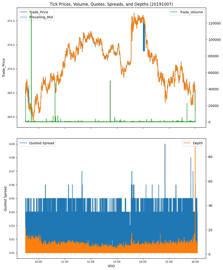
The data is preprocessed to extract a universe of U.S.-domiciled common stocks, and indexed by ticker symbol for efficient access.

for d, date in enumerate(dates):
    store = Store(storedir / str(date), verbose=VERBOSE)
    master, trades, quotes = opentaq(date, taqdir)

    # screen on CRSP universe
    univ = crsp.get_universe(date)\
               .join(crsp.get_section(dataset='names',
                                      fields=['ncusip', 'permco', 'exchcd'],
                                      date_field='date',
                                      date=date,
                                      start=0), how='inner')\
               .sort_values(['permco', 'ncusip'])

    # drop duplicate share classes (same permco): keep largest cap
    dups = master['CUSIP'].str\
                          .slice(0, 8)\
                          .isin(univ.loc[univ.duplicated(['permco'],keep=False),
                                         'ncusip'])
    #shareclass.extend(master[dups].to_dict(orient='index').values())    
    univ = univ.sort_values(['permco', 'cap'], na_position='first')\
               .drop_duplicates(['permco'], keep='last')\
               .reset_index()\
               .set_index('ncusip', drop=False)

    # Iterate by symbol over Daily Taq trades, nbbo and master files
    for ct, cq, mast in itertaq(trades,
                                quotes,
                                master,
                                cusips=univ['ncusip'],
                                open_t=open_t,
                                close_t=None,
                                verbose=VERBOSE):
        header = {'date':date}
        header.update(univ.loc[mast['CUSIP'][:8],
                               ['permno','decile','exchcd','siccd']])
        header.update(mast[['Symbol', 'Round_Lot']])
        store[header['Symbol']] = dict(header=header, ct=ct, cq=cq, mast=mast)
    quotes.close()
    trades.close()

Liquidty measures

• Depth: The average bid and ask size at the best quotes, indicating the available liquidity at the current market price.

• Quoted Spread: The difference between the best ask and best bid prices, representing the cost of immediacy for traders.

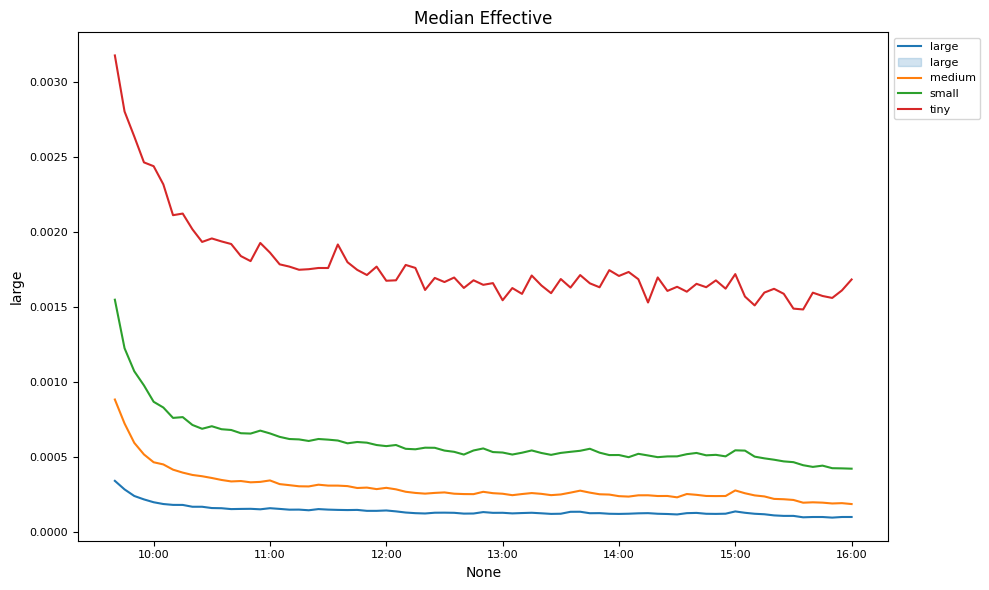
• Effective Spread: A trade-based measure of execution cost, calculated as twice the absolute difference between the trade price and the midquote.

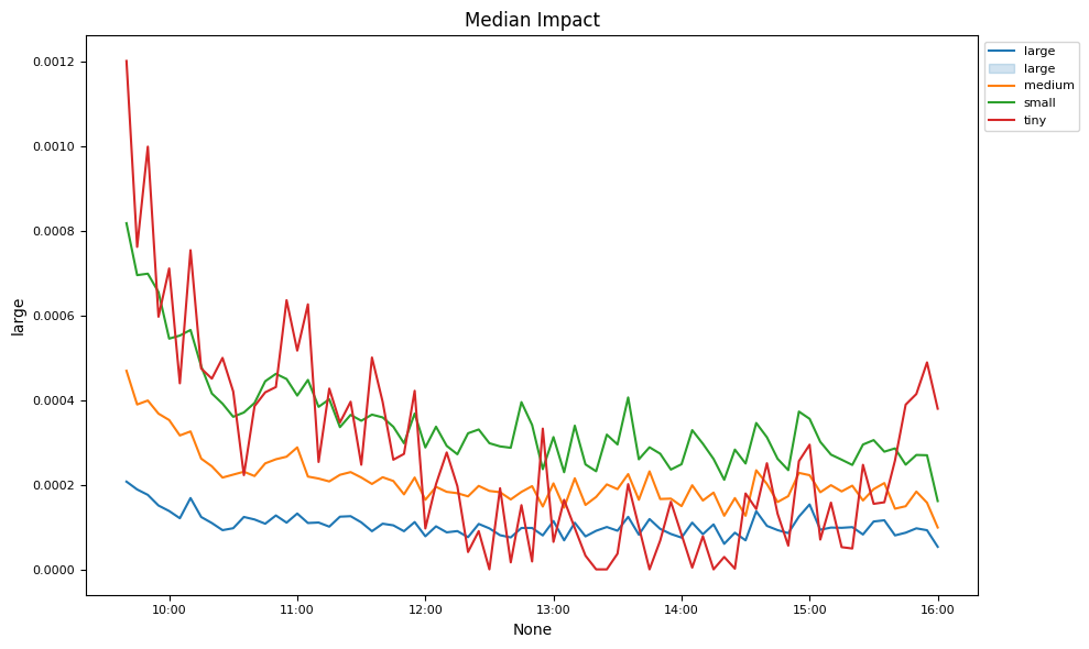
• Price Impact: The change in the midquote price after a trade, reflecting how much a trade moves the market.

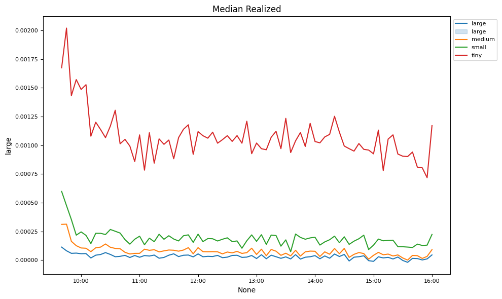
• Realized Spread: The difference between the trade price and the midquote price a few minutes later, measuring the profitability of liquidity providers.

• Lee-Ready Tick Test: A method for classifying trades as buyer- or seller-initiated, using trade price movements relative to the prevailing midquote.

• Volume Weighted Average Price (VWAP) – A common trade execution benchmark, though it can be influenced by the trade itself – achieving zero slippage to VWAP while accounting for 100% of market volume does not necessarily indicate good execution.

Intraday liquidity

Intraday liquidity is analyzed computing liquidity measures across various time intervals: 1-second, 2-second, 5-second, 15-second, 30-second, 1-minute, 2-minute, and 5-minute bins.

intervals = ([(v, 's') for v in [1, 2, 5, 15, 30]] + [(v, 'm') for v in [1, 2, 5]])
max_num = 100000
bin_keys = ['effective', 'realized', 'impact',
            'quoted', 'volume', 'offersize', 'bidsize',
            'ret', 'retq', 'counts']

# helper call run liquidity calculations by date, parallelizable
def intraday(date):
    """Compute intraday liquidity for a date"""
    store = Store(storedir / str(date), verbose=VERBOSE)
    symbols = sorted(store)
    daily_all = []
    bins_all = {k: [] for k in bin_keys}
    for num, symbol in enumerate(symbols):
        if num >= max_num:    # set small max_num for debugging
            break
        header, ct, cq, mast = store[symbol].values()

        # Compute and collect daily and bin statistics at all intervals
        daily = header.copy()   # to collect current stock's daily stats

        # Compute effective spreads by large and small trade sizes
        med_volume = mast['Round_Lot'] * (cq['Best_Bid_Size'].median()
                                          + cq['Best_Offer_Size'].median()) / 2.
        data = ct.loc[(ct.index > open_t) & (ct.index < close_t),
                      ['Trade_Price', 'Prevailing_Mid', 'Trade_Volume']]
        eff_spr = data['Trade_Price'].div(data['Prevailing_Mid']).sub(1).abs()
        eff_large = eff_spr[data['Trade_Volume'].ge(med_volume).to_numpy()]
        daily['large_trades'] = len(eff_large)
        daily['large_volume'] = data.loc[data['Trade_Volume'].ge(med_volume),
                                'Trade_Volume'].mean()
        daily['large_spread'] = eff_large.mean()
        eff_small = eff_spr[data['Trade_Volume'].lt(med_volume)]
        daily['small_trades'] = len(eff_small)
        daily['small_volume'] = data.loc[data['Trade_Volume'].lt(med_volume),
                                'Trade_Volume'].mean()
        daily['small_spread'] = eff_small.mean()

        v, u = intervals[-1]
        for (v, u) in intervals:
            bt = bin_trades(ct, v, u, open_t=open_t, close_t=close_t)
            bq = bin_quotes(cq, v, u, open_t=open_t, close_t=close_t)
            daily[f"tvar{v}{u}"] = bt['ret'].var(ddof=0) * len(bt)
            daily[f"tvarHL{v}{u}"] = ((hl_vol(bt['maxtrade'], bt['mintrade'])**2)
                                      * len(bt))
            daily[f"tvarOHLC{v}{u}"] = ((ohlc_vol(bt['first'],
                                                  bt['maxtrade'],
                                                  bt['mintrade'],
                                                  bt['last'])**2)
                                        * len(bt))
            daily[f"qvar{v}{u}"] = bq['retq'].var(ddof=0) * len(bq)
            daily[f"qvarHL{v}{u}"] = ((hl_vol(bq['maxmid'], bq['minmid'])**2)
                                      * len(bq))
            daily[f"qvarOHLC{v}{u}"] = ((ohlc_vol(bq['firstmid'],
                                                  bq['maxmid'],
                                                  bq['minmid'],
                                                  bq['mid'])**2)
                                        * len(bq))
            daily[f"tunch{v}{u}"] = np.mean(np.abs(bt['ret']) < EPSILON)
            daily[f"qunch{v}{u}"] = np.mean(np.abs(bq['retq']) < EPSILON)
            daily[f"tzero{v}{u}"] = np.mean(bt['counts'] == 0)


        # Collect final (i.e. 5 minute bins) bt and bq intraday series
        df = bq.join(bt, how='left')
        for s in ['effective', 'realized', 'impact', 'quoted']:
            bins_all[s].append({**header,
                                **(df[s]/df['mid']).to_dict()})
        for s in ['volume', 'offersize', 'bidsize', 'ret', 'retq', 'counts']:
            bins_all[s].append({**header,
                                **df[s].to_dict()})

        # Collect daily means
        daily.update(df[['bidsize', 'offersize', 'quoted', 'mid']].mean())
        daily.update(df[['volume', 'counts']].sum())
        daily.update(weighted_average(df[['effective', 'impact', 'realized',
                                            'vwap', 'volume']],
                                        weights='volume'))
        daily_all.append(daily)
        
    return DataFrame(daily_all), {k: DataFrame(bins_all[k]) for k in bin_keys}

To optimize performance, multiprocessing package is used to parallelize computations, allowing efficient distribution of input data across multiple processes using its Pool API.

# Run each day as a parallel thread, must be called as context manager or with close command
with multiprocessing.Pool(processes=min(os.cpu_count(), len(dates))) as p:
    data = p.map(intraday, dates)

# Combine data
daily_df = pd.concat([data[j][0] for j in range(len(data))], ignore_index=True)
bins_df = {k: pd.concat([data[j][1][k] for j in range(len(data))], ignore_index=True)
           for k in bin_keys}

# Store in scratch folder
store = Store(paths['scratch'])

store['tick.daily'] = daily_df
store['tick.bins'] = bins_df

# Fetch extracted data    
daily_df = store['tick.daily']
bins_df = store['tick.bins']

By market capitalization

The daily averages of liquidity measures are analyzed across different market capitalization categories.

# group by market cap (NYSE deciles 1-3, 4-6, 7-9, 10) and exchange listed
daily_df['Size'] = pd.cut(daily_df['decile'],
                          [0, 3.5, 6.5, 9.5, 11],
                          labels=['large', 'medium', 'small', 'tiny'])
groupby = daily_df.groupby(['Size'], observed=False)

# collect results for each metric
results = {}    # to collect results as dict of {column: Series}
formats = {}    # and associated row formatter string
results.update(groupby['mid']\
               .count()\
               .rename('Number of Stock/Days').to_frame())
formats.update({'Number of Stock/Days': '{:.0f}'})

result = groupby[['mid', 'vwap']].mean()   # .quantile(), and range
result.columns = ['Midquote Price', "VWAP"]
formats.update({k: '{:.2f}' for k in result.columns})
results.update(result)

result = groupby[['counts', 'volume']].mean()
result.columns = ['Number of trades', "Volume (shares)"]
formats.update({k: '{:.0f}' for k in result.columns})
results.update(result)

# volatility from 5m intervals
result = np.sqrt(groupby[['tvar5m', 'qvar5m', 'tvarHL5m', 'qvarHL5m',
                          'tvarOHLC5m', 'qvarOHLC5m']].mean())
result.columns = ['Volatility(trade price)', "Volatility(midquote)",
                  'Volatility(HL trade price)', "Volatility(HL midquote)",
                  'Volatility(OHLC trade price)', "Volatility(OHLC midquote)"]
formats.update({k: '{:.4f}' for k in result.columns})
results.update(result)

result = groupby[['offersize', 'bidsize']].mean()
result.columns = [s.capitalize() + ' (lots)' for s in result.columns]
formats.update({k: '{:.1f}' for k in result.columns})
results.update(result)

spr = ['quoted', 'effective', 'impact', 'realized']
result = groupby[spr].mean()
result.columns = [s.capitalize() + ' $ spread' for s in spr]
formats.update({k: '{:.4f}' for k in result.columns})
results.update(result)

rel = [s.capitalize() + ' (% price)' for s in spr]
daily_df[rel] = daily_df[spr].div(daily_df['mid'], axis=0)  # scale spreads
result = 100*groupby[rel].mean()
formats.update({k: '{:.4f}' for k in result.columns})
results.update(result)

# summarize large and small trade effective spreads
spr = ['large_spread', 'small_spread']
result = 100*groupby[spr].mean()
result.columns = ['Large trade (% spread) ', 'Small trade (% spread) ']
formats.update({k: '{:.4f}' for k in result.columns})
results.update(result)

spr = ['large_trades', 'small_trades']
result = groupby[spr].mean()
result.columns = ['Large trade (# trades) ', 'Small trade (# trades) ']
formats.update({k: '{:.0f}' for k in result.columns})
results.update(result)

spr = ['large_volume', 'small_volume']
result = groupby[spr].mean()
result.columns = ['Large trade (avg volume) ', 'Small trade (avg volume) ']
formats.update({k: '{:.0f}' for k in result.columns})
results.update(result)

# display table of results
print("Average Liquidity by Market Cap")
row_formatted(DataFrame(results).T, formats)

Average Liquidity by Market Cap

Size	large	medium	small	tiny
Number of Stock/Days	2063	2572	4297	4618
Midquote Price	128.98	64.91	27.76	7.92
VWAP	128.97	64.92	27.75	7.90
Number of trades	25178	8407	3658	837
Volume (shares)	3031056	995483	533736	254773
Volatility(trade price)	0.0145	0.0211	0.0359	0.0807
Volatility(midquote)	0.0152	0.0223	0.0355	0.0918
Volatility(HL trade price)	0.0176	0.0217	0.0335	0.0690
Volatility(HL midquote)	0.0144	0.0198	0.0288	0.0594
Volatility(OHLC trade price)	0.0184	0.0218	0.0324	0.0612
Volatility(OHLC midquote)	0.0138	0.0183	0.0255	0.0452
Offersize (lots)	8.8	9.8	11.9	13.6
Bidsize (lots)	8.9	17.0	14.1	16.5
Quoted $ spread	0.0630	0.0672	0.0781	0.0841
Effective $ spread	0.0379	0.0442	0.0406	0.0457
Impact $ spread	0.0273	0.0244	0.0248	0.0186
Realized $ spread	0.0106	0.0199	0.0158	0.0270
Quoted (% price)	0.0350	0.0834	0.2500	1.1582
Effective (% price)	0.0200	0.0421	0.1287	0.6638
Impact (% price)	0.0165	0.0345	0.0904	0.2669
Realized (% price)	0.0036	0.0077	0.0384	0.3973
Large trade (% spread)	0.0191	0.0420	0.1310	0.6398
Small trade (% spread)	0.0190	0.0400	0.1304	0.6755
Large trade (# trades)	3133	1140	423	108
Small trade (# trades)	22045	7267	3236	729
Large trade (avg volume)	1734	1608	2635	2324
Small trade (avg volume)	61	57	71	85

By time of day

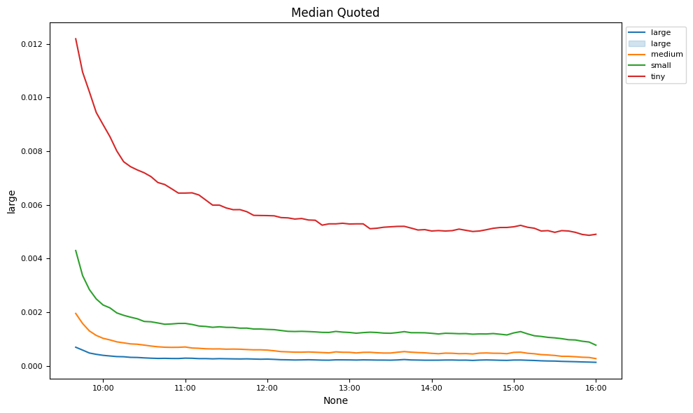
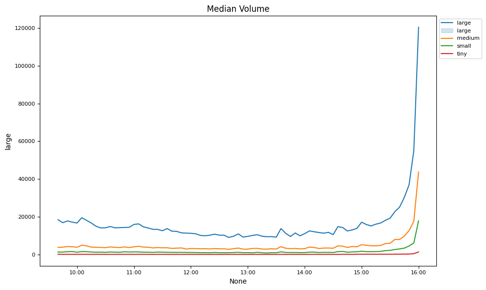
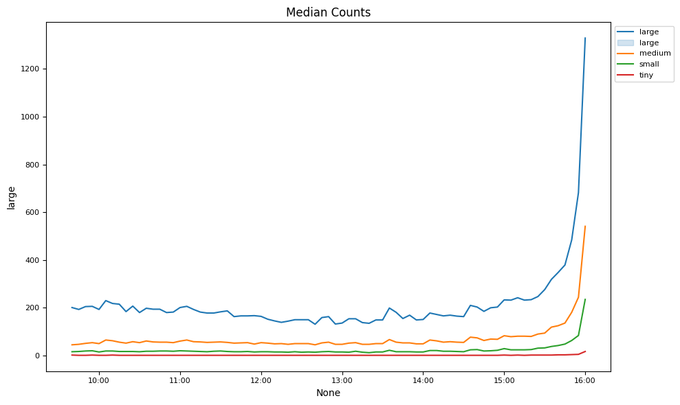
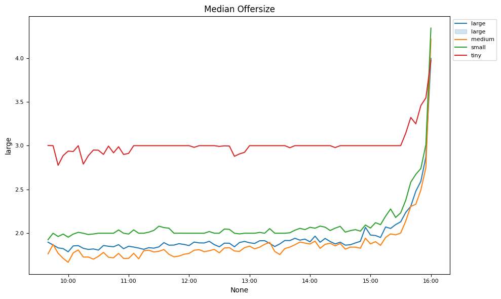
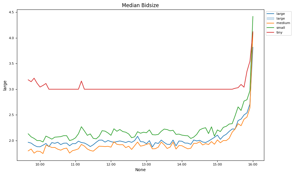
Market liquidity changes are examined over the trading day.

# Plot intraday spreads, depths and volumes
keys = ['effective', 'realized', 'impact', 'quoted', 
        'volume', 'counts', 'offersize', 'bidsize']
for num, key in enumerate(keys):
    df = bins_df[key].drop(columns=['Round_Lot', 'Symbol'])
    df.index = list(zip(df['permno'], df['date']))
        
    # Group by market cap
    df['Size'] = pd.cut(df['decile'],
                        [0, 3.5, 6.5, 9.5, 11],
                        labels=['large', 'medium', 'small', 'tiny'])
    df = df.drop(columns=['date', 'permno', 'decile', 'exchcd', 'siccd'])\
           .dropna()\
           .groupby(['Size'], observed=False)\
           .median().T
    fig, ax = plt.subplots(1, 1, num=num+1, clear=True, figsize=(10, 6))
    plot_time(df.iloc[1:], ax=ax, fontsize=8)
    ax.legend(['large'] + list(df.columns), 
              loc='upper left', bbox_to_anchor=(1.0, 1.0), 
              fontsize=8)
    ax.set_title('Median ' + key.capitalize())
    plt.subplots_adjust(right=0.8)
    plt.tight_layout()

High frequency sampling

Variance ratio

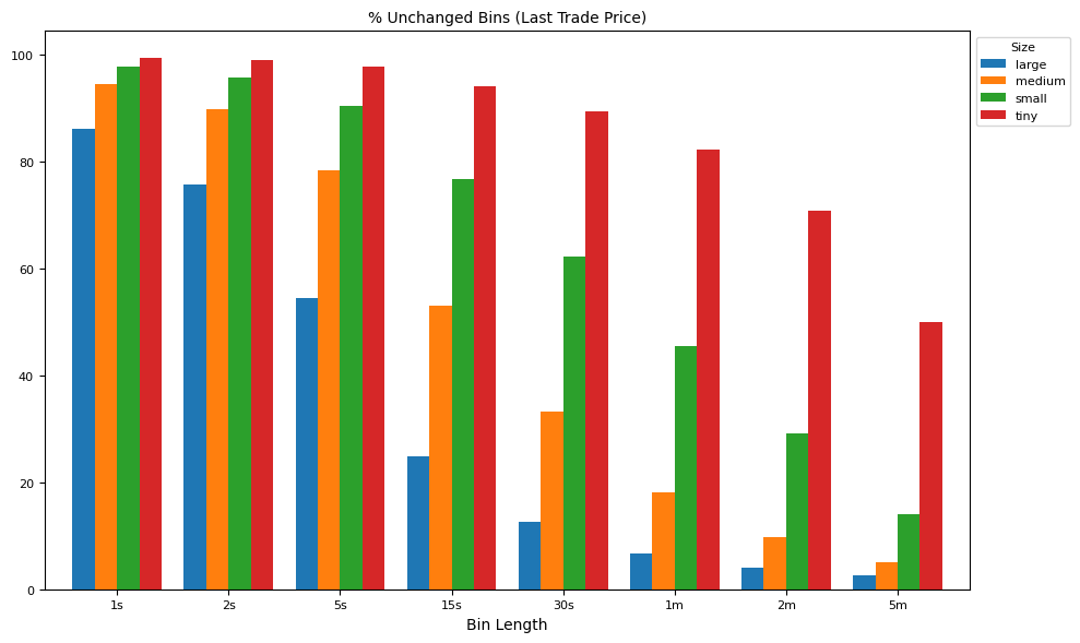
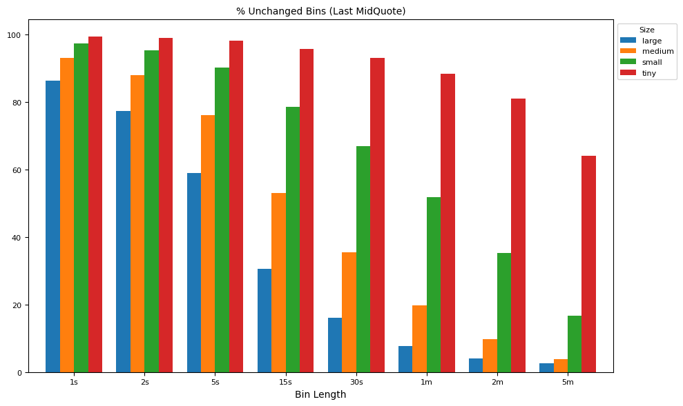
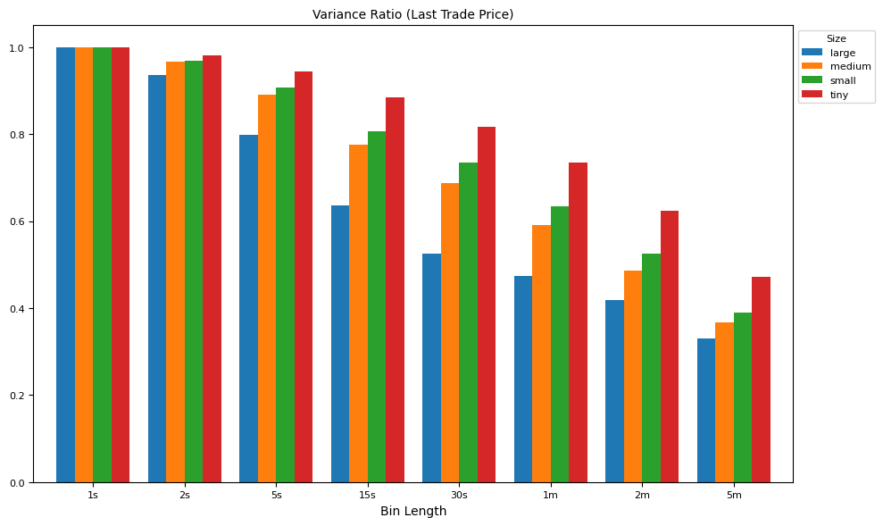
Tick data often exhibits spurious autocorrelation due to irregularly spaced trades and quotes rather than continuous trading:

• Non-Continuous Trading: Trades and quotes occur discretely, often clustering around news or market events.

• Order Flow Clustering: Market participants submit bursts of orders, creating short-term price autocorrelation.

• Bid-Ask Bounce: Trades alternate between the bid and ask prices, creating an illusion of mean-reverting returns.

The variance ratio test (Lo & MacKinlay, 1988) checks for mean reversion or momentum by comparing **multi-period return variance to single-period return variance, scaled by the number of periods.

def plot_helper(result, xticks, keys, legend, xlabel, title, ylim=[],
                figsize=(10, 6), num=1, fontsize=8):
    """helper to plot bar graphs by sampling frequency"""
    fig, ax = plt.subplots(num=num, clear=True, figsize=figsize)
    result.plot(kind='bar',
                fontsize=fontsize,
                rot=0,
                width=0.8,
                xlabel='',
                ax=ax)
    if ylim:
        ax.set_ylim(*ylim)
    ax.set_xticklabels(xticks, fontsize=fontsize)
    ax.legend(keys, loc='upper left', bbox_to_anchor=(1.0, 1.0), 
              fontsize=fontsize, title=legend, title_fontsize=8)
    ax.set_xlabel(xlabel, fontsize=fontsize + 2)
    ax.set_title(title, fontsize=fontsize + 2)
    plt.subplots_adjust(right=0.8, bottom=0.15)
    plt.tight_layout()
    return ax

xticks = [f"{v}{u}" for v, u in intervals]   # x-axis: bin lengths
keys = list(groupby.indices.keys())          # legend labels

labels = [f"tunch{v}{u}" for v, u in intervals]
result = groupby[labels].median()*100
ax = plot_helper(result.T,
                 title="% Unchanged Bins (Last Trade Price)",
                 xticks=xticks,
                 xlabel="Bin Length",
                 keys=keys,
                 legend='Size',
                 num=1)

labels = [f"qunch{v}{u}" for v, u in intervals]
result = groupby[labels].median()*100
ax = plot_helper(result.T,
                 title="% Unchanged Bins (Last MidQuote)",
                 xticks=xticks,
                 xlabel="Bin Length",
                 keys=keys,
                 legend='Size',
                 num=2)

labels = [f"tzero{v}{u}" for v, u in intervals]
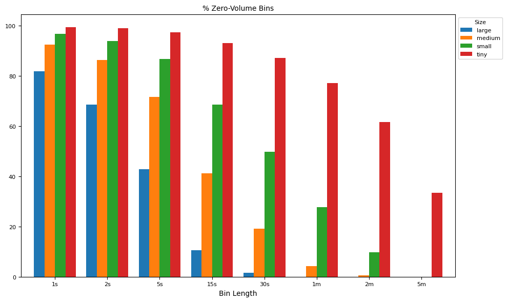
result = groupby[labels].median()*100
ax = plot_helper(result.T,
                 title="% Zero-Volume Bins",
                 xticks=xticks,
                 xlabel="Bin Length",
                 keys=keys,
                 legend='Size',
                 num=3)

labels = [f"tvar{v}{u}" for v, u in intervals]
result = groupby[labels].median()
result = result.div(result['tvar1s'].values, axis=0)
ax = plot_helper(result.T,
                 title="Variance Ratio (Last Trade Price)",
                 xticks=xticks,
                 xlabel="Bin Length",
                 keys=keys,
                 legend='Size',
                 num=4)

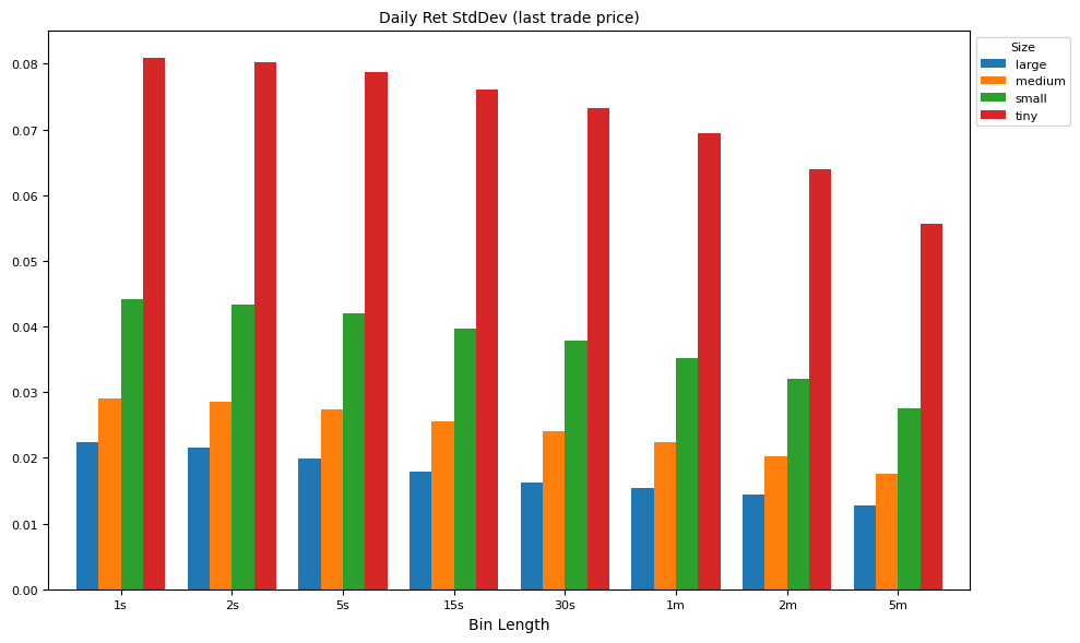
labels = [f"tvar{v}{u}" for v, u in intervals]
result = np.sqrt(groupby[labels].median())
ax = plot_helper(result.T,
                 title="Daily Ret StdDev (last trade price)",
                 xticks=xticks,
                 xlabel="Bin Length",
                 keys=keys,
                 legend='Size',
                 num=5)

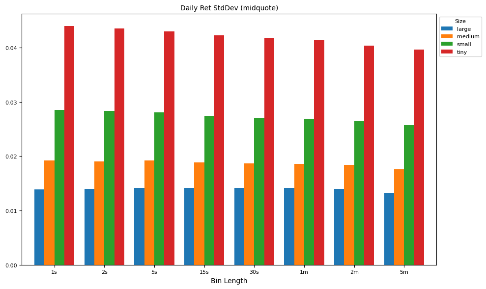
labels = [f"qvar{v}{u}" for v, u in intervals]
result = np.sqrt(groupby[labels].median())
ax = plot_helper(result.T,
                 title="Daily Ret StdDev (midquote)",
                 xticks=xticks,
                 xlabel="Bin Length",
                 keys=keys,
                 legend='Size',
                 num=6)

Volatility measures

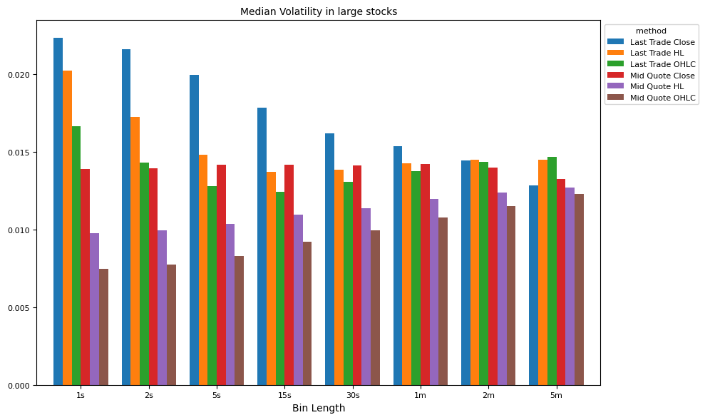
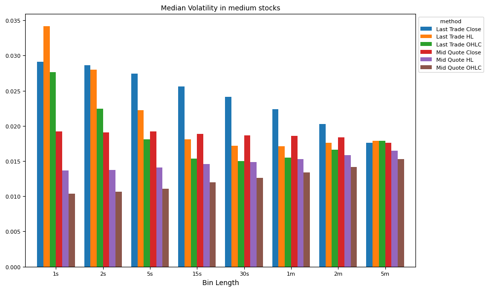
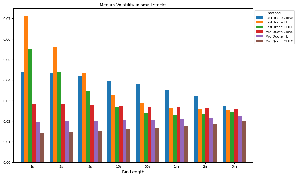
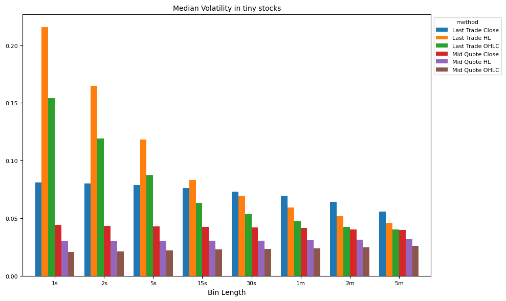
Parkinson’s (HL) Volatility estimator uses the high-low price range to estimate volatility, assuming a geometric Brownian motion without a drift term:
$\( \sigma_{HL} = \frac{\sqrt{\ln 2}}{\sqrt{4T\ln 2}} \times \frac{\text{H} - \text{L}}{\sqrt{\Delta t}} \)$

This method is more efficient than close-to-close volatility but assumes continuous trading and no jumps.

The Klass-Garman (OHLC) Volatility estimator improves on Parkinson’s by incorporating open, high, low, and close prices for better accuracy:
$\( \sigma^2_{OHLC} = 0.511 (H - L)^2 - 0.019 (C - O)(H + L - 2O) - 0.383 (C - O)^2 \)$

This model accounts for both overnight jumps and intra-day movements.

# Compare methods of volatility estimates, by interval and market cap
for ifig, (split_label, split_df) in enumerate(groupby):
    vol_df = np.sqrt(split_df[[c for c in daily_df.columns if "qvar" in c or "tvar" in c]])
    result = []
    for col in [c for c in vol_df.columns if "qvar" in c or "tvar" in c]:
        if col[4] == 'H':
            m = 'HL'
        elif col[4] == 'O':
            m = 'OHLC'
        else:
            m = 'Close'
        result.append({'method': {'t': 'Last Trade', 'q': 'Mid Quote'}[col[0]] + ' ' + m,
                       'interval': (int("".join(filter(str.isdigit, col)))
                                    * (60 if col[-1] == 'm' else 1)),
                       'val': vol_df[col].median()})
    result = DataFrame.from_dict(result, orient='columns')\
        .pivot(index='interval', columns='method', values='val')\
        .sort_index()
    ax = plot_helper(result,
                     title="Median Volatility in " + " ".join(split_label) + " stocks",
                     xticks=xticks,
                     xlabel="Bin Length",
                     keys=result.columns,
                     num=ifig+1,
                     legend='method')

References:

Andrew W. Lo, A. Craig MacKinlay, Stock Market Prices Do Not Follow Random Walks: Evidence from a Simple Specification Test, The Review of Financial Studies, Volume 1, Issue 1, January 1988, Pages 41–66, https://doi.org/10.1093/rfs/1.1.41

Parkinson, M. (1980) The Extreme Value Method for Estimating the Variance of the Rate of Return. Journal of Business, 53, 61-65. http://dx.doi.org/10.1086/296071