Industry Community Detection

Realize that everything connects to everything else - Leonardo DaVinci

Traditional industry classification systems, such as SIC and NAICS, group firms based on production processes or product similarities. Natural language processing techniques can be leveraged to analyze product descriptions and capture dynamic changes in industry structures over time, as proposed by Hoberg and Phillips (2016). Industry communities can be detected through network analysis, where firms are modeled as nodes in a graph, and connections between them are determined by similarities in their product and market descriptions.

# By: Terence Lim, 2020-2025 (terence-lim.github.io)
import zipfile
import io
from itertools import chain
import numpy as np
import pandas as pd
from pandas import DataFrame, Series
import matplotlib.pyplot as plt
import seaborn as sns
import networkx as nx
from finds.database import SQL
from finds.readers import requests_get, Sectoring
from finds.structured import BusDay, PSTAT
from finds.recipes import graph_info
from secret import credentials
# %matplotlib qt
VERBOSE = 0

sql = SQL(**credentials['sql'], verbose=VERBOSE)
bd = BusDay(sql)
pstat = PSTAT(sql, bd, verbose=VERBOSE)

Industry taxonomy

Industry classification, or industry taxonomy, organizes companies into groups based on shared characteristics such as production processes, product offerings, or financial market behaviors.

Text-based industry classification

Hoberg and Phillips (2016) developed a text-based measure of firm similarity by analyzing product descriptions in 10-K filings. They construct firm-by-firm similarity scores using word vectors, filtering out common words and focusing on nouns and proper nouns, while excluding geographic terms. The similarity between firms is quantified using cosine similarity, creating a pairwise similarity matrix across firms and years.

Since Item 101 of Regulation S-K mandates that firms accurately describe their key products in their 10-K filings, the TNIC scheme, based on textual similarity, provides a dynamic classification system that evolves with market changes. This method offers a more flexible alternative to traditional classification systems, capturing shifts in product markets over time.

Source: Hoberg and Phillips Industry Classification

The TNIC pair-wise firm similiarities are retrieved from the Hoberg and Phillips website:

# Retrieve TNIC scheme from Hoberg and Phillips website
tnic_scheme = 'tnic3'
root = 'https://hobergphillips.tuck.dartmouth.edu/idata/'   
source = root + tnic_scheme + '_data.zip'
if source.startswith('http'):
    response = requests_get(source)
    source = io.BytesIO(response.content)

# extract the csv file from zip archive
with zipfile.ZipFile(source).open(tnic_scheme + "_data.txt") as f:
    tnic_data = pd.read_csv(f, sep='\s+')

# extract latest year of tnic as data frame
year = max(tnic_data['year']) # [1989, 1999, 2009, 2019]
tnic = tnic_data[tnic_data['year'] == year].dropna()
tnic

	year	gvkey1	gvkey2	score
26307358	2023	1004	1823	0.0127
26307359	2023	1004	4091	0.0087
26307360	2023	1004	5567	0.0063
26307361	2023	1004	9698	0.0075
26307362	2023	1004	10519	0.0191
...	...	...	...	...
26973403	2023	351038	329141	0.0684
26973404	2023	351038	331856	0.0769
26973405	2023	351038	332115	0.1036
26973406	2023	351038	347007	0.0731
26973407	2023	351038	349972	0.0871

666050 rows × 4 columns

Industry classification

Industry classification systems such as SIC and NAICS follow hierarchical structures to categorize firms based on their economic activities:

• Standard Industrial Classification (SIC): Uses a 2-digit, 3-digit, and 4-digit hierarchy to classify industries.

• North American Industry Classification System (NAICS): Expands classification granularity from 2-digit to 6-digit levels.

# populate dataframe of nodes with gvkey (as index), permno, sic and naics
nodes = DataFrame(index=sorted(set(tnic['gvkey1']).union(tnic['gvkey2'])))\
        .rename_axis(index='gvkey')
for code in ['lpermno', 'sic', 'naics']:
    lookup = pstat.build_lookup('gvkey', code, fillna=0)
    nodes[code] = lookup(nodes.index)
Series(np.sum(nodes > 0, axis=0)).rename('Non-missing').to_frame().T

	lpermno	sic	naics
Non-missing	3829	3829	3827

# supplement naics and sic with crosswalks in Sectoring class
naics = Sectoring(sql, 'naics', fillna=0)   # supplement from crosswalk
sic = Sectoring(sql, 'sic', fillna=0)
nodes['naics'] = nodes['naics'].where(nodes['naics'] > 0, naics[nodes['sic']])
nodes['sic'] = nodes['sic'].where(nodes['sic'] > 0, sic[nodes['naics']])
Series(np.sum(nodes > 0, axis=0)).rename('Non-missing').to_frame().T 

	lpermno	sic	naics
Non-missing	3829	3829	3829

Sector groups

Industry taxonomies group detailed classifications into broader sectors for economic analysis:

• Fama and French aggregate 4-digit SIC codes into industry groups consisting of 5, 10, 12, 17, 30, 38, 48, or 49 sectors.

• The Bureau of Economic Analysis (BEA) consolidates 6-digit NAICS codes into summary-level industry groups, with updates in 1947, 1963, and 1997.

# include sectoring schemes
codes = {'sic': ([f"codes{c}" for c in [5, 10, 12, 17, 30, 38, 48, 49]]
                 + ['sic2', 'sic3']),
         'naics': ['bea1947', 'bea1963', 'bea1997']}
sectorings = {}   # store Sectoring objects
for key, schemes in codes.items():
    for scheme in schemes:
        if scheme not in sectorings:

            # missing value is integer 0 sic2 and sic3 shemes, else string ''
            fillna = 0 if scheme.startswith('sic') else ''

            # load the sectoring class from SQL
            sectorings[scheme] = Sectoring(sql, scheme, fillna=fillna)

            # apply the sectoring scheme to partition the nodes
            nodes[scheme] = sectorings[scheme][nodes[key]]

        # keep nodes with non-missing data
        nodes = nodes[nodes[scheme].ne(sectorings[scheme].fillna)]
        print(len(nodes), scheme)
nodes

3845 codes5
3845 codes10
3845 codes12
3845 codes17
3845 codes30
3845 codes38
3845 codes48
3845 codes49
3829 sic2
3829 sic3
3561 bea1947
3561 bea1963
3561 bea1997

	lpermno	sic	naics	codes5	codes10	codes12	codes17	codes30	codes38	codes48	codes49	sic2	sic3	bea1947	bea1963	bea1997
gvkey
1004	54594	5080	423860	Cnsmr	Shops	Shops	Machn	Whlsl	Whlsl	Whlsl	Whlsl	50	508	42	42	42
1045	21020	4512	481111	Other	Durbl	Durbl	Trans	Trans	Trans	Trans	Trans	45	451	48	481	481
1050	11499	3564	333413	Manuf	Manuf	Manuf	Machn	FabPr	Machn	Mach	Mach	35	356	333	333	333
1076	10517	6141	522220	Other	Other	Money	Finan	Fin	Money	Banks	Banks	61	614	52	521CI	521CI
1078	20482	3845	334510	Hlth	Hlth	Hlth	Other	Hlth	Instr	MedEq	MedEq	38	384	334	334	334
...	...	...	...	...	...	...	...	...	...	...	...	...	...	...	...	...
345980	20333	5961	455110	Cnsmr	Shops	Shops	Rtail	Rtail	Rtail	Rtail	Rtail	59	596	44RT	44RT	4A0
347007	15533	2836	325414	Hlth	Hlth	Hlth	Other	Hlth	Chems	Drugs	Drugs	28	283	325	325	325
349337	20867	3845	334510	Hlth	Hlth	Hlth	Other	Hlth	Instr	MedEq	MedEq	38	384	334	334	334
349972	15642	2836	325414	Hlth	Hlth	Hlth	Other	Hlth	Chems	Drugs	Drugs	28	283	325	325	325
351038	16161	2834	325412	Hlth	Hlth	Hlth	Cnsum	Hlth	Chems	Drugs	Drugs	28	283	325	325	325

3561 rows × 16 columns

Community structure

In network analysis, community structure refers to the clustering of nodes (firms) into partitions (groups) based on connectivity patterns. Identifying these communities helps reveal hidden industry relationships and competitive dynamics.

# populate undirected graph with tnic edges
edges = tnic[tnic['gvkey1'].isin(nodes.index) & tnic['gvkey2'].isin(nodes.index)]
edges = list(
    edges[['gvkey1', 'gvkey2', 'score']].itertuples(index=False, name=None))
G = nx.Graph()
G.add_weighted_edges_from(edges)
G.remove_edges_from(nx.selfloop_edges(G))  # remove self-loops: not necessary
Series(graph_info(G, fast=True)).rename(year).to_frame()

	2023
transitivity	0.877035
average_clustering	0.575643
connected	False
connected_components	9
size_largest_component	3523
directed	False
weighted	True
negatively_weighted	False
edges	320352
nodes	3541
selfloops	0
density	0.051113

Measuring partitions

The quality of graph partitions can be evaluated using modularity, a measure that assesses the strength of community structures by comparing observed connections within clusters to a random network model.

# evaluate modularity of sectoring schemes on TNIC graph
def community_quality(G, communities):
    """helper to measure quality of partitions"""
    out = {'communities': len(communities)}
    out['modularity'] = nx.community.modularity(G, communities)
    (out['coverage'],
     out['performance']) = nx.community.partition_quality(G, communities)    
    return out

modularity = {}   # to collect measurements of each scheme
for scheme in sorted(chain(*codes.values())):
    communities = nodes.loc[list(G.nodes), scheme]\
                       .reset_index()\
                       .groupby(scheme)['gvkey']\
                       .apply(list)\
                       .to_list()    # list of lists of node labels
    modularity[scheme] = community_quality(G, communities)
df = DataFrame.from_dict(modularity, orient='index').sort_index()
print(f"Quality of sectoring schemes on TNIC graph ({year})")
df

Quality of sectoring schemes on TNIC graph (2023)

	communities	modularity	coverage	performance
bea1947	40	0.330481	0.779187	0.925859
bea1963	58	0.324246	0.734745	0.948296
bea1997	61	0.324169	0.734514	0.948689
codes10	10	0.335843	0.940503	0.850069
codes12	12	0.336655	0.938187	0.878268
codes17	17	0.285847	0.766719	0.794675
codes30	30	0.335544	0.934385	0.899115
codes38	36	0.333800	0.793237	0.890785
codes48	48	0.331168	0.752610	0.944559
codes49	49	0.331003	0.751526	0.951096
codes5	5	0.337074	0.945045	0.818984
sic2	67	0.327541	0.743694	0.942476
sic3	226	0.288389	0.690952	0.958297

Detecting partitions

Community detection in graphs can be performed using various algorithms, including:

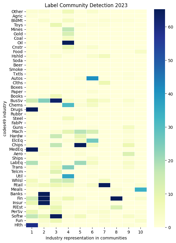
• Label Propagation Algorithm: This method assigns an initial label to each node and iteratively updates labels based on the majority of its neighbors’ labels, allowing communities to form dynamically. It is fast and works well for large networks but may produce different results on different runs due to randomness.

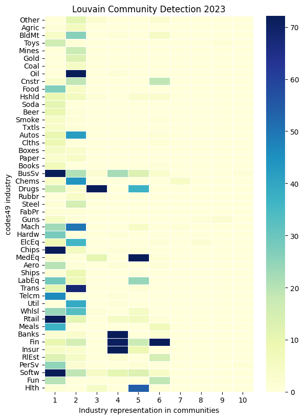
• Louvain Method: This hierarchical clustering algorithm optimizes modularity by iteratively merging small communities into larger ones, maximizing intra-community connections while minimizing inter-community edges.

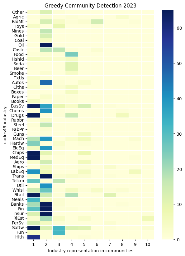
• Greedy Algorithm: This algorithm builds communities by iteratively merging pairs of nodes or groups that result in the largest modularity gain, prioritizing locally optimal choices.

# Run community detection algorithms
def community_detection(G):
    """Helper to run community detection algorithms on an undirected graph"""
    out = {}
    out['label'] = nx.community.label_propagation_communities(G)
    out['louvain'] = nx.community.louvain_communities(G, resolution=1)
    out['greedy'] = nx.community.greedy_modularity_communities(G, resolution=1)
    return out

communities = community_detection(G)
quality = {}
for key, community in communities.items():
    quality[key] = community_quality(G, community)

df = DataFrame.from_dict(quality, orient='index').sort_index()
print(f"Modularity of community detection algorithms on TNIC graph ({year})")
df

Modularity of community detection algorithms on TNIC graph (2023)

	communities	modularity	coverage	performance
greedy	51	0.323848	0.989711	0.689093
label	101	0.347795	0.990485	0.909486
louvain	19	0.354818	0.824855	0.838868

# Visualize Fama-French 49-industries in the detected communities
key = 'codes49'
for ifig, detection in enumerate(communities.keys()):

    # count industries represented in each partition
    industry = []
    communities_sequence = sorted(communities[detection], key=len, reverse=True)    
    for i, community in enumerate(communities_sequence):
        industry.append(nodes[key][list(community)].value_counts().rename(i+1))
    names = sectorings[key].sectors['name'].drop_duplicates(keep='first')
    df = pd.concat(industry, axis=1)\
           .dropna(axis=0, how='all')\
           .fillna(0)\
           .astype(int)\
           .reindex(names)

    # display as heatmap
    fig, ax = plt.subplots(num=ifig+1, clear=True, figsize=(6, 8))
    sns.heatmap(df.iloc[:,:10],
                square=False,
                linewidth=.5,
                ax=ax,
                yticklabels=1,
                cmap="YlGnBu",
                robust=True)
    if scheme.startswith('bea'):
        ax.set_yticklabels(Sectoring._bea_industry[df.index], size=10)
    else:
        ax.set_yticklabels(df.index, size=10)
    ax.set_title(f'{detection.capitalize()} Community Detection {year}')
    ax.set_xlabel(f"Industry representation in communities")
    ax.set_ylabel(f"{key} industry")
    fig.subplots_adjust(left=0.4)
    plt.tight_layout(pad=0)

References

Gerard Hoberg and Gordon Phillips, 2016, Text-Based Network Industries and Endogenous Product Differentiation.Journal of Political Economy 124 (5), 1423-1465.

Gerard Hoberg and Gordon Phillips, 2010, Product Market Synergies and Competition in Mergers and Acquisitions: A Text-Based Analysis. Review of Financial Studies 23 (10), 3773-3811.