Machine Learning: Regression

Whereof what’s past is prologue - Shakespeare

We explore supervised machine learning and regression models for macroeconomic forecasting, with a focus on predicting the industrial production index (INDPRO) using a wide range of economic indicators. To improve generalization and predictive performance, we investigate methods such as subset selection, penalized regression, decision trees, and ensemble learning, aiming to strike a balance between model complexity and accuracy.

# By: Terence Lim, 2020-2025 (terence-lim.github.io)
import numpy as np
import pandas as pd
from pandas import DataFrame, Series
import matplotlib.pyplot as plt
import statsmodels.api as sm
from sklearn.metrics import mean_squared_error    
from finds.readers.alfred import Alfred, fred_md
from finds.utils import plot_date
from secret import credentials
# %matplotlib qt
VERBOSE = 0

Macroeconomic forecasting

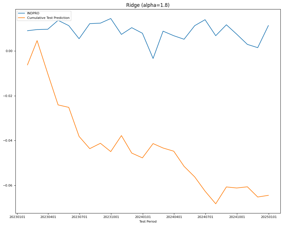
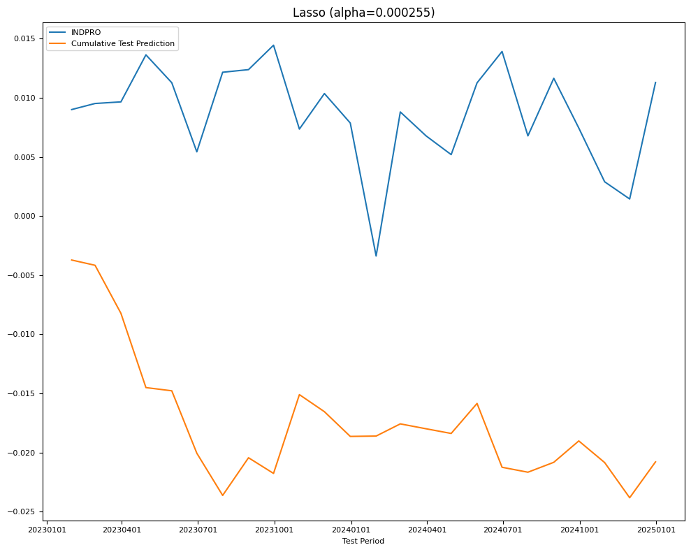
For the candidate regression models, the independent variables consist of up to three lags of each economic indicator. The objective is to predict the rate of change in the industrial production index (INDPRO) for the following month while minimizing the mean squared error (MSE) loss function, which is appropriate for continuous-valued targets.

Monthly macroeconomic data is retrieved from FRED-MD, with any missing recent values supplemented from other public sources. Suggested transformations are applied to each time series to ensure stationarity. The pre-2023 period is used for training, while the post-2023 period is reserved for testing.

alf = Alfred(api_key=credentials['fred']['api_key'], verbose=-1)

# Get latest FRED-MD data
freq = 'M' 
beg = 19640701  # 19620701
df, t = fred_md()   # 
transforms = t['transform']
end = df.index[-2]
split_date = end - 20000
print("Train/test date ranges:", beg, split_date, end)

FRED-MD vintage: monthly/current.csv
Train/test date ranges: 19640701 20221231 20241231

# Splice in common updates: source of PE ratio, Commercial Paper
for col in ['S&P PE ratio']:
    df[col] = alf.splice(col)
df['COMPAPFF'] = df['COMPAPFF'].ffill()  # forward fill 20200430
df['CP3M'] = df['CP3M'].ffill()          # forward fill 20200430

# Apply time series transformations according to FRED-MD
transformed = []
for col in df.columns:
    transformed.append(alf.transform(df[col], tcode=transforms[col], freq=freq))
data = pd.concat(transformed, axis=1).iloc[2:]
c = list(data.columns)
data = data.loc[(data.index >= beg) & (data.index <= end)]

# Drop columns with missing data
missing = []
for series_id in df.columns:
    g = data[series_id].notna()
    missing.extend([(date, series_id) for date in data.index[~g]])
missing_per_row = data.isna().sum(axis=1)
missing = DataFrame.from_records(missing, columns=['date', 'series_id'])
print('original:', data.shape, 'dropna:', data.dropna(axis=1).shape)
data = data.dropna(axis=1)   # drop columns where missing values
print(missing['series_id'].value_counts())
data

original: (726, 126) dropna: (726, 122)
series_id
ACOGNO          332
UMCSENT         163
TWEXAFEGSMTH    103
ANDENO           44
Name: count, dtype: int64

	RPI	W875RX1	DPCERA3M086SBEA	CMRMTSPL	RETAIL	INDPRO	IPFPNSS	IPFINAL	IPCONGD	IPDCONGD	...	DDURRG3M086SBEA	DNDGRG3M086SBEA	DSERRG3M086SBEA	CES0600000008	CES2000000008	CES3000000008	DTCOLNVHFNM	DTCTHFNM	INVEST	VIXCLS
19640731	0.005422	0.005404	0.007343	0.019986	0.004947	0.006552	0.010342	0.011313	0.014079	0.016438	...	0.000667	-0.000369	-0.000090	-0.000016	0.003231	-0.004158	-0.003798	-0.002430	-0.002831	11.2238
19640831	0.005644	0.006061	0.005992	-0.020139	0.013974	0.006506	-0.000936	-0.000939	-0.001865	0.007219	...	-0.002031	-0.002398	0.001406	-0.000016	-0.003263	0.004141	-0.005958	-0.001818	0.011673	13.6898
19640930	0.004123	0.004205	-0.004164	0.027173	0.009372	0.003703	-0.004690	-0.003759	-0.011267	-0.023656	...	0.000728	0.003749	-0.001674	-0.000015	-0.006462	0.004090	-0.011142	-0.003802	0.010582	10.5167
19641031	0.000555	0.000650	0.006499	-0.013866	-0.039421	-0.013947	-0.010404	-0.013269	-0.020030	-0.109875	...	-0.001712	-0.002344	0.000525	-0.011757	0.016093	-0.024760	0.005974	-0.000704	-0.003579	11.0924
19641130	0.006703	0.007352	-0.009111	-0.009745	0.009335	0.030429	0.029043	0.031929	0.036884	0.128121	...	0.004137	0.000985	-0.000352	0.011772	-0.019272	0.024828	-0.009946	-0.002806	-0.002694	12.0087
...	...	...	...	...	...	...	...	...	...	...	...	...	...	...	...	...	...	...	...	...	...
20240831	0.000066	-0.000117	0.000711	0.000375	-0.001144	0.004869	0.004515	0.007094	0.009218	0.047547	...	0.000600	-0.002222	-0.000061	-0.002580	0.001376	-0.006110	-0.001974	-0.000766	0.001445	19.6750
20240930	0.001458	0.000240	0.005257	0.007155	0.008903	-0.004205	-0.005809	-0.008928	-0.002317	-0.001441	...	0.005721	-0.002598	0.000553	0.004137	0.001906	0.004652	-0.002368	-0.001586	-0.001644	17.6597
20241031	0.003690	0.003488	0.001757	-0.001714	0.005575	-0.004547	-0.007220	-0.010970	-0.006158	-0.028598	...	-0.002965	0.003609	0.000788	-0.003839	-0.005006	-0.002154	-0.000146	0.003227	-0.000473	19.9478
20241130	0.002184	0.002756	0.004346	0.003993	0.006484	-0.001453	-0.001180	-0.000155	-0.004246	0.018794	...	-0.000986	0.000117	-0.002176	-0.000639	-0.002760	0.003190	-0.000872	-0.001679	-0.011753	15.9822
20241231	0.001234	0.001391	0.005441	0.006665	0.007175	0.009853	0.007300	0.006569	0.003359	-0.013311	...	-0.004215	0.004218	0.002086	0.002521	0.005776	-0.001439	0.002963	0.002748	0.002421	15.6997

726 rows × 122 columns

Data beyond the split date is excluded from model training to ensure a proper evaluation of generalization performance.

# Split time series train and test set
def ts_split(X, Y, end=split_date):
    """helper to split train/test time series"""
    return X[Y.index<=end], X[Y.index>end], Y[Y.index<=end], Y[Y.index>end]

def columns_map(columns, lag):
    """helper to create lagged column names"""
    return {col: col + '_' + str(lag) for col in columns}

def columns_unmap(columns):
    """helper to extract lagged column names"""
    cols = [col.split('_') for col in columns]
    return [col[0] for col in cols], [int(col[1]) for col in cols]

target_id = 'INDPRO'
lags = 3   # Include up to 3 lags of exogs
Y = data[target_id].iloc[lags:]
X = pd.concat([data.shift(lag).iloc[lags:]\
               .rename(columns=columns_map(data.columns, lag))
               for lag in range(1, lags+1)],
              axis=1)
                      

# new table to collect final fitted models
test = Series(name='test', dtype=float)    # collect test and train errors
train = Series(name='train', dtype=float)
final_models = {}  

Regression models

Complex regression models with numerous features or parameters risk overfitting, capturing noise rather than true patterns. Several techniques help mitigate overfitting and improve model generalization:

• Cross-validation: Hyperparameter tuning using cross-validation helps ensure models generalize well across different data subsets. K-fold Cross-Validation (K-fold CV) divides the dataset into \(K\) parts, training the model on \(K-1\) sections and testing it on the remaining part, iterating through all folds and averaging results. Leave-One-Out Cross-Validation (LOOCV) is a special case where each data point serves as the test set once, helping refine hyperparameter selection.

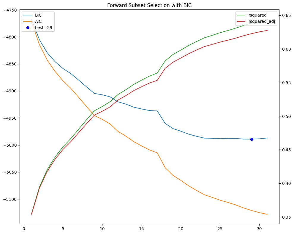
• Information criteria penalty: The Akaike Information Criterion (AIC) and Bayesian Information Criterion (BIC) aid model selection by balancing goodness of fit and complexity. AIC, defined as \(AIC = 2k - 2\ln(L)\), where \(k\) is the number of parameters and \(L\) is the likelihood, favors models that explain the data with minimal complexity. BIC, given by \(BIC = k\ln(n) - 2\ln(L)\), introduces a stronger penalty for sample size \(n\), preferring simpler models for large datasets. Lower AIC or BIC values indicate better models.

• Ensemble learning: By combining multiple weak learners, ensemble methods enhance model robustness. Bagging averages predictions from multiple models trained on different data subsets, reducing variance. Boosting sequentially corrects model errors, improving overall accuracy.

Forward Subset Selection

Forward Subset Regression is a stepwise variable selection method used in regression modeling to identify the best subset of predictors. It begins with no variables in the model and iteratively adds the most significant predictor at each step, based on a chosen criterion, and stops when adding more variables does not significantly improve model performance. Penalized selection criteria, such as AIC or BIC, helps avoid overfitting. Forward selection is computationally more efficient than exhaustive search methods but may miss the optimal subset if an initially excluded variable becomes relevant later in combination with others.

def forward_select(Y, X, selected, ic='aic'):
    """helper to forward select next regressor, using sm.OLS"""
    remaining = [x for x in X.columns if x not in selected]
    results = []
    for x in remaining:
        r = sm.OLS(Y, X[selected + [x]]).fit()
        results.append({'select': x,
                        'aic': r.aic,
                        'bic': r.bic,
                        'rsquared': r.rsquared,
                        'rsquared_adj': r.rsquared_adj})
    return DataFrame(results).sort_values(by=ic).iloc[0].to_dict()

# find best bic, and show selection criteria scores
ic = 'bic'   # select by information criterion
X_train, X_test, Y_train, Y_test = ts_split(X, Y)
selected = []
models = {}
for i in range(1, 32):
    select = forward_select(Y_train,
                            X_train,
                            selected,
                            ic=ic)
    models[i] = select
    selected.append(select['select'])
selected = DataFrame.from_dict(models, orient='index')
best = selected[[ic]].iloc[selected[ic].argmin()]
subset = selected.loc[:best.name].round(3)
subset.index = [alf.header(s.split('_')[0]) for s in subset['select']]
print('Forward Selection Subset')
subset

Forward Selection Subset

	select	aic	bic	rsquared	rsquared_adj
Initial Claims	CLAIMS_1	-4772.162	-4767.612	0.355	0.354
Real M2 Money Stock	M2REAL_2	-4814.414	-4805.315	0.394	0.393
All Employees, Wholesale Trade	USWTRADE_2	-4843.063	-4829.414	0.420	0.418
All Employees, Service-Providing	SRVPRD_2	-4864.114	-4845.916	0.439	0.436
5-Year Treasury Constant Maturity Minus Federal Funds Rate	T5YFFM_3	-4881.249	-4858.500	0.454	0.450
Total Business: Inventories to Sales Ratio	ISRATIO_2	-4895.191	-4867.893	0.467	0.462
All Employees, Service-Providing	SRVPRD_1	-4911.828	-4879.981	0.481	0.475
All Employees, Financial Activities	USFIRE_2	-4928.888	-4892.490	0.495	0.489
All Employees, Trade, Transportation, and Utilities	USTPU_1	-4945.576	-4904.629	0.508	0.502
Consumer Motor Vehicle Loans Owned by Finance Companies, Level	DTCOLNVHFNM_3	-4952.630	-4907.133	0.514	0.507
Industrial Production: Nondurable Energy Consumer Goods: Residential Utilities	IPB51222S_3	-4960.975	-4910.928	0.521	0.514
Industrial Production: Nondurable Goods Materials	IPNMAT_3	-4974.770	-4920.175	0.532	0.524
Canadian Dollars to U.S. Dollar Spot Exchange Rate	EXCAUS_3	-4983.489	-4924.343	0.539	0.531
M1	M1SL_3	-4993.678	-4929.983	0.547	0.538
Nonrevolving consumer credit to Personal Income	CONSPI_2	-5001.564	-4933.319	0.554	0.544
Market Yield on U.S. Treasury Securities at 10-Year Constant Maturity, Quoted on an Investment Basis	GS10_1	-5008.976	-4936.181	0.560	0.549
Capacity Utilization: Manufacturing (SIC)	CUMFNS_2	-5014.366	-4937.022	0.564	0.553
Industrial Production: Manufacturing (SIC)	IPMANSICS_2	-5041.837	-4959.943	0.582	0.571
All Employees, Nondurable Goods	NDMANEMP_1	-5056.048	-4969.605	0.592	0.580
Average Hourly Earnings of Production and Nonsupervisory Employees, Construction	CES2000000008_1	-5065.393	-4974.400	0.598	0.586
Average Weekly Overtime Hours of Production and Nonsupervisory Employees, Manufacturing	AWOTMAN_2	-5075.474	-4979.931	0.605	0.593
Industrial Production: Equipment: Business Equipment	IPBUSEQ_2	-5083.967	-4983.875	0.611	0.598
Industrial Production: Total Index	INDPRO_2	-5091.928	-4987.286	0.617	0.604
Real Estate Loans, All Commercial Banks	REALLN_1	-5096.759	-4987.568	0.620	0.607
All Employees, Mining, Quarrying, and Oil and Gas Extraction	CES1021000001_2	-5102.029	-4988.288	0.624	0.610
Moody's Seasoned Baa Corporate Bond Yield	BAA_1	-5106.126	-4987.835	0.627	0.613
Moody's Seasoned Aaa Corporate Bond Yield	AAA_1	-5110.792	-4987.951	0.631	0.616
All Employees, Mining, Quarrying, and Oil and Gas Extraction	CES1021000001_1	-5116.399	-4989.008	0.635	0.620
Industrial Production: Materials	IPMAT_1	-5120.986	-4989.046	0.638	0.623

DataFrame.from_dict({n: {'series_id': s.split('_')[0],
                         'lag' : s.split('_')[1],
                         'description': alf.header(s.split('_')[0])}
                     for n, s in selected.loc[:best.name, 'select'].items()},
                    orient='index').set_index('series_id')

	lag	description
series_id
CLAIMS	1	Initial Claims
M2REAL	2	Real M2 Money Stock
USWTRADE	2	All Employees, Wholesale Trade
SRVPRD	2	All Employees, Service-Providing
T5YFFM	3	5-Year Treasury Constant Maturity Minus Federa...
ISRATIO	2	Total Business: Inventories to Sales Ratio
SRVPRD	1	All Employees, Service-Providing
USFIRE	2	All Employees, Financial Activities
USTPU	1	All Employees, Trade, Transportation, and Util...
DTCOLNVHFNM	3	Consumer Motor Vehicle Loans Owned by Finance ...
IPB51222S	3	Industrial Production: Nondurable Energy Consu...
IPNMAT	3	Industrial Production: Nondurable Goods Materials
EXCAUS	3	Canadian Dollars to U.S. Dollar Spot Exchange ...
M1SL	3	M1
CONSPI	2	Nonrevolving consumer credit to Personal Income
GS10	1	Market Yield on U.S. Treasury Securities at 10...
CUMFNS	2	Capacity Utilization: Manufacturing (SIC)
IPMANSICS	2	Industrial Production: Manufacturing (SIC)
NDMANEMP	1	All Employees, Nondurable Goods
CES2000000008	1	Average Hourly Earnings of Production and Nons...
AWOTMAN	2	Average Weekly Overtime Hours of Production an...
IPBUSEQ	2	Industrial Production: Equipment: Business Equ...
INDPRO	2	Industrial Production: Total Index
REALLN	1	Real Estate Loans, All Commercial Banks
CES1021000001	2	All Employees, Mining, Quarrying, and Oil and ...
BAA	1	Moody's Seasoned Baa Corporate Bond Yield
AAA	1	Moody's Seasoned Aaa Corporate Bond Yield
CES1021000001	1	All Employees, Mining, Quarrying, and Oil and ...
IPMAT	1	Industrial Production: Materials

# Plot BIC vs number selected
fig, ax = plt.subplots(num=1, figsize=(10, 8))
selected['bic'].plot(ax=ax, c='C0')
selected['aic'].plot(ax=ax, c='C1')
ax.plot(best.name, float(best.iloc[0]), "ob")
ax.legend(['BIC', 'AIC', f"best={best.name}"], loc='upper left')
ax.set_title(f"Forward Subset Selection with {ic.upper()}")
bx = ax.twinx()
selected['rsquared'].plot(ax=bx, c='C2')
selected['rsquared_adj'].plot(ax=bx, c='C3')
bx.legend(['rsquared', 'rsquared_adj'], loc='upper right')
bx.set_xlabel('# Predictors')
plt.tight_layout()

# evaluate train and test mse
X_subset = X_train[subset['select']]
model = sm.OLS(Y_train, X_subset).fit()
name = f"Forward Subset Regression (k={len(subset)})"
Y_pred = model.predict(X_test[subset['select']])
test[name] = mean_squared_error(Y_test, Y_pred)                               
train[name] = mean_squared_error(Y_train, model.predict(X_subset))
final_models[name] = model

fig, ax = plt.subplots(figsize=(10, 8))
plot_date(pd.concat([Y_test.cumsum(), Y_pred.cumsum()], axis=1),
          legend1=[target_id, 'Cumulative Test Prediction'],
          title=name,
          xlabel='Test Period',
          fontsize=8,
          ax=ax)
plt.tight_layout()

DataFrame({'name': name,
           'train': np.sqrt(train[name]),
           'test': np.sqrt(test[name])}, index=['RMSE'])

	name	train	test
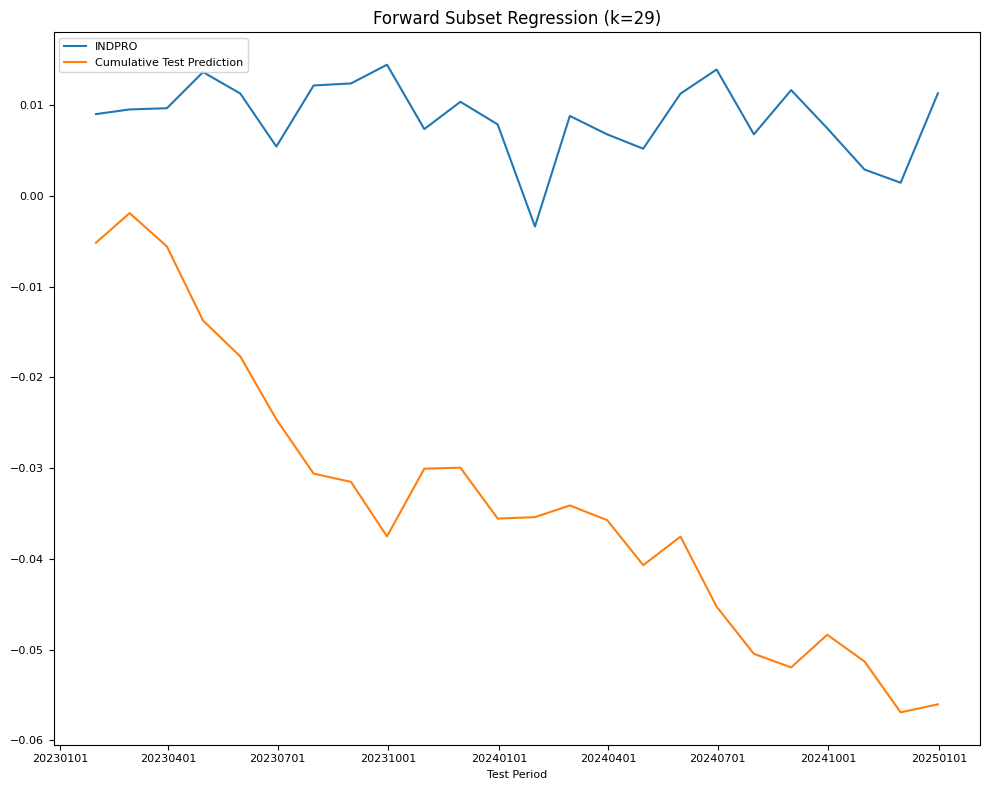
RMSE	Forward Subset Regression (k=29)	0.005955	0.007674

Partial Least Squares Regression

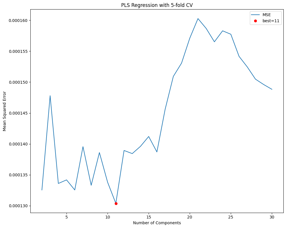
Partial Least Squares (PLS) Regression combines features of principal component analysis (PCA) and multiple linear regression. PLS constructs new latent variables (components) as linear combinations of the original predictors that maximize covariance with the response variable. The number of components (n_components) parameter controls the dimensionality reduction and must be chosen carefully to balance bias-variance tradeoff. This method is particularly useful when datasets have more predictors than observations and strong multicollinearity.

# split train and test, fit standard scaling using train set
from sklearn.preprocessing import StandardScaler
from sklearn.cross_decomposition import PLSRegression
from sklearn.model_selection import cross_val_score, KFold
X_train, X_test, Y_train, Y_test = ts_split(X, Y)
scale = StandardScaler().fit(X_train)
X_train = scale.transform(X_train)
X_test = scale.transform(X_test)

# fit with 5-fold CV to choose n_components
n_splits=5
kf = KFold(n_splits=n_splits, shuffle=True, random_state=0)
mse = Series(dtype=float)
for i in np.arange(2, 31):
    pls = PLSRegression(n_components=i)
    score = cross_val_score(estimator=pls,
                            X=X_train,
                            y=Y_train,
                            n_jobs=5,
                            verbose=VERBOSE,
                            cv=kf,
                            scoring='neg_mean_squared_error').mean()
    mse.loc[i] = -score

# show cross-validation results and best model
fig, ax = plt.subplots(figsize=(10, 8))
mse.plot(ylabel='Mean Squared Error',
         xlabel='Number of Components',
         title=f"PLS Regression with {n_splits}-fold CV",
         ax=ax)
best = mse.index[mse.argmin()]
ax.plot(best, mse.loc[best], "or")
ax.legend(['MSE', f"best={best}"])
plt.tight_layout()

### evaluate train and test mse
model = PLSRegression(n_components=best).fit(X_train, Y_train)
name = f"PLS Regression(k={best})"
Y_pred = Series(index=Y_test.index,
                data=model.predict(X_test).reshape((-1,)))

test[name] = mean_squared_error(Y_test, Y_pred)
train[name] = mean_squared_error(Y_train, model.predict(X_train))
final_models[name] = model

fig, ax = plt.subplots(figsize=(10, 8))
plot_date(pd.concat([Y_test.cumsum(), Y_pred.cumsum()], axis=1),
          legend1=[target_id, 'Cumulative Test Prediction'],
          title=name,
          xlabel='Test Period',
          fontsize=8,
          ax=ax)
plt.tight_layout()

DataFrame({'name': name,
           'train': np.sqrt(train[name]),
           'test': np.sqrt(test[name])}, index=['RMSE'])

	name	train	test
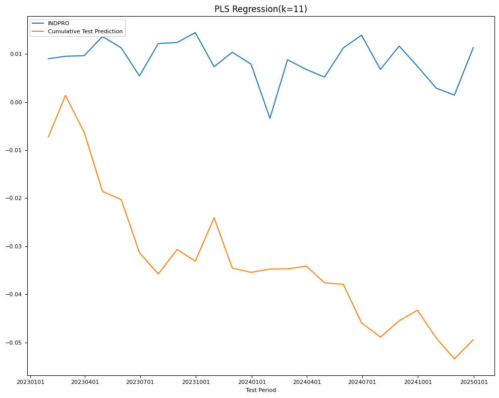
RMSE	PLS Regression(k=11)	0.005306	0.008791

Ridge Regression

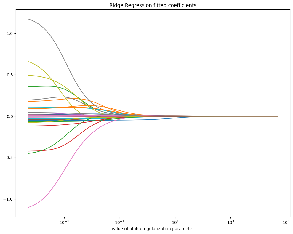
Ridge Regression is a linear regression model that includes L2 regularization, which helps prevent overfitting by adding a penalty term to the loss function. The objective function is modified as follows:

\[ \min_w ||y - Xw||^2 + \lambda ||w||^2 \]

where \(||y - Xw||^2\) is the standard least squares error, and \(\lambda ||w||^2\) is the penalty term that shrinks the model coefficients \(w\) towards zero. The \(\lambda\) parameter (alpha in sklearn’s Ridge) controls the strength of regularization: larger values reduce model complexity by forcing coefficients to be smaller, while smaller values make Ridge behave like standard linear regression. Ridge retains all features but reduces their impact, which is useful when dealing with multicollinearity, without completely eliminating any predictor.

from sklearn.linear_model import Ridge, RidgeCV
alphas = 10**np.linspace(5, -4, 100)*0.5  # for parameter tuning
X_train, X_test, Y_train, Y_test = ts_split(X, Y)
scale = StandardScaler().fit(X_train)
X_train = scale.transform(X_train)
X_test = scale.transform(X_test)
np.random.seed(42)

# Plot fitted coefficients vs regularization alpha
coefs = [Ridge(alpha, fit_intercept=False)\
         .fit(X_subset, Y_train).coef_ for alpha in alphas]
fig, ax = plt.subplots(figsize=(10, 8))
ax.plot(alphas, coefs)
ax.set_xscale('log')
ax.set_xlabel('value of alpha regularization parameter')
ax.set_title('Ridge Regression fitted coefficients')
plt.tight_layout()

# RidgeCV LOOCV
model = RidgeCV(alphas=alphas,
                scoring='neg_mean_squared_error',
                cv=None,  # to use Leave-One-Out cross validation
                store_cv_values=True).fit(X_train, Y_train)

name = f"Ridge (alpha={model.alpha_:.1f})"
Y_pred = Series(index=Y_test.index,
                data=model.predict(X_test).reshape((-1,)))
test[name] = mean_squared_error(Y_test, Y_pred)
train[name] = mean_squared_error(Y_train, model.predict(X_train))
final_models[name] = model

fig, ax = plt.subplots(figsize=(10, 8))
plot_date(pd.concat([Y_test.cumsum(), Y_pred.cumsum()], axis=1),
          legend1=[target_id, 'Cumulative Test Prediction'],
          title=name,
          xlabel='Test Period',
          fontsize=8,
          ax=ax)
plt.tight_layout()

DataFrame({'name': name,
           'train': np.sqrt(train[name]),
           'test': np.sqrt(test[name])}, index=['RMSE'])

	name	train	test
RMSE	Ridge (alpha=1.8)	0.004305	0.009825

Lasso Regression

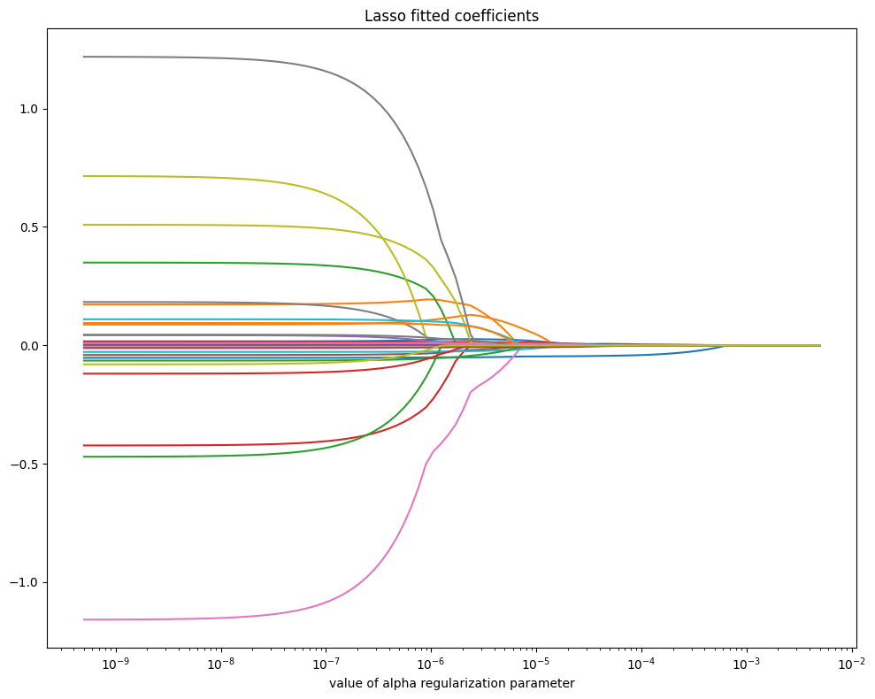
Lasso Regression (Least Absolute Shrinkage and Selection Operator) is a linear regression model that includes L1 regularization, which adds the sum of the absolute values of the coefficients as a penalty term to the loss function. This encourages sparsity, meaning it shrinks some coefficients to exactly zero, effectively performing feature selection. The objective function is:

\[ \min_w ||y - Xw||^2_2 + \alpha ||w||_1 \]

where \(\alpha\) is a hyperparameter controlling the strength of regularization: a higher \(\alpha\) increases shrinkage, leading to more coefficients being set to zero. Lasso regression is particularly useful when dealing with high-dimensional data where many features may be irrelevant, by reducing model complexity and improving interpretability. However, with correlated features, it tends to arbitrarily select one and ignore the others.

from sklearn.linear_model import Lasso, LassoCV
alphas = 10**np.linspace(-2, -9, 100)*0.5  # for parameter tuning
X_train, X_test, Y_train, Y_test = ts_split(X, Y)
scale = StandardScaler().fit(X_train)
X_train = scale.transform(X_train)
X_test = scale.transform(X_test)

# Plot fitted coefficients vs regularization
coefs = [Lasso(max_iter=10000, alpha=alpha)\
         .fit(X_subset, Y_train).coef_  for alpha in alphas]
fig, ax = plt.subplots(figsize=(10, 8))
ax.plot(alphas, coefs)
ax.set_xscale('log')
ax.set_xlabel('value of alpha regularization parameter')
ax.set_title('Lasso fitted coefficients')
plt.tight_layout()

# LassoCV 10-Fold CV
model = LassoCV(alphas=None,
                cv=5,
                n_jobs=5,
                verbose=VERBOSE,
                max_iter=20000).fit(X_train, Y_train)
name = f"Lasso (alpha={model.alpha_:.3g})"
Y_pred = Series(index=Y_test.index,
                data=model.predict(X_test).reshape((-1,)))
test[name] = mean_squared_error(Y_test, Y_pred)
train[name] = mean_squared_error(Y_train, model.predict(X_train))
final_models[name] = model

fig, ax = plt.subplots(figsize=(10, 8))
plot_date(pd.concat([Y_test.cumsum(), Y_pred.cumsum()], axis=1),
          legend1=[target_id, 'Cumulative Test Prediction'],
          title=name,
          xlabel='Test Period',
          fontsize=8,
          ax=ax)
plt.tight_layout()

DataFrame({'name': name,
           'train': np.sqrt(train[name]),
           'test': np.sqrt(test[name])}, index=['RMSE'])

	name	train	test
RMSE	Lasso (alpha=0.000255)	0.006279	0.006808

# Display nonzero coefs
nonzero = np.sum(np.abs(model.coef_) > 0)
argsort = np.flip(np.argsort(np.abs(model.coef_)))[:nonzero]
df = DataFrame({'series_id': columns_unmap(X.columns[argsort])[0],
                'lags': columns_unmap(X.columns[argsort])[1],
                'desc': [alf.header(s)
                         for s in columns_unmap(X.columns[argsort])[0]],
                'coef': model.coef_[argsort]}).round(6).set_index('series_id')
print("Lasso: Nonzero Coefficients")
df

Lasso: Nonzero Coefficients

	lags	desc	coef
series_id
CLAIMS	1	Initial Claims	-0.005356
SRVPRD	1	All Employees, Service-Providing	-0.001268
M2REAL	2	Real M2 Money Stock	0.000893
IPNMAT	3	Industrial Production: Nondurable Goods Materials	0.000751
USGOVT	1	All Employees, Government	-0.000716
...	...	...	...
M2SL	3	M2	0.000020
COMPAPFF	3	3-Month Commercial Paper Minus FEDFUNDS	-0.000020
UEMPLT5	3	Number Unemployed for Less Than 5 Weeks	0.000019
CUSR0000SAS	3	Consumer Price Index for All Urban Consumers: ...	0.000009
RPI	3	Real Personal Income	0.000002

82 rows × 3 columns

Decision Tree

Decision trees partition the predictor space into regions, making predictions based on mean values (for regression) or mode (for classification).

• A decision tree consists of a sequence of splitting rules that divide observations into different regions. These trees are typically drawn upside down, with the leaves at the bottom.

• Terminal nodes or leaves represent the final partitions of the predictor space where observations are grouped.

• Internal nodes are points in the tree where the predictor space is split.

• Branches connect the nodes and represent different decision paths.

• A stump refers to a decision tree with only a single split (one internal node).

Decision trees are constructed using recursive binary splitting, a top-down, greedy algorithm. The process begins with all observations in a single region, and at each step, the predictor space is split into two new branches based on the best possible split at that moment (without considering future steps). The best split is determined by selecting the predictor and cutpoint that minimize a chosen cost function, such as the Residual Sum of Squares (RSS) in regression. The process continues recursively until a stopping criterion is met, such as a minimum number of observations per node.

Growing a tree until all leaves are pure (containing only one class) often leads to overfitting. Tree complexity is measured by the number of nodes, and controlling this complexity is crucial. If trees are allowed to grow too large, they may fit the training data well but perform poorly on unseen data. A balance must be found where accuracy on the test set is maximized before further tree growth begins to decrease performance.

Overfitting can be mitigated by pruning the tree using cost complexity pruning. A fully grown tree is simplified by removing less important splits to minimize the following function:

\[\sum_{m=1}^{|T|} \sum_{x_i \in R_m} (y_i - \hat{y}_{R_m})^2 + \alpha |T| \]

where \(|T|\) is the number of terminal nodes, \(R_m\) represents a region in the predictor space, and \(\hat{y}_{R_m}\) is the predicted response for that region. Pruning is controlled by a tuning parameter \(\alpha\), where higher values result in smaller trees that generalize better.

For classification tasks, different impurity measures determine the best binary splits:

• Classification error rate: Measures the proportion of incorrectly classified observations in a node. While intuitive, it is not sensitive enough for effective tree growth.

\[ \hat{\rho}_{m,c} = \frac{n_{m,c}}{n_m} \]

where \(n_m\) is the number of observations in node \(m\) and \(n_{m,c}\) is the number of observations in node \(m\) belonging to class \(c\).

• Gini index: Measures total variance across classes. A lower Gini index indicates that most observations in a node belong to a single class.

\[ G = \sum_{k=1}^{K} \hat{\rho}_{mk} (1 - \hat{\rho}_{mk}) \]

where \(\hat{\rho}_{mk}\) represents the proportion of training observations in node \(m\) that belong to class \(k\).

• Entropy: Measures node impurity. Lower entropy values indicate purer nodes.

\[ D = -\sum_{k=1}^{K} \hat{\rho}_{mk} \log \hat{\rho}_{mk} \]

Deviance is a statistical measure used to assess model performance in classification problems. It is derived from the likelihood function and is a measure of how well the predicted probabilities match the actual class labels. It is calculated as:

\[ Deviance = -2 \sum_{m=1}^{g} \sum_{c=1}^{w} n_{m,c} \ln \hat{p}_{m,c} \]

where:

• \(g\) is the number of terminal nodes (leaf nodes) in the forest.

• \(w\) is the number of classes.

• \(n_{m,c}\) is the number of observations in node \(m\) belonging to class \(c\).

• \(\hat{p}_{m,c}\) is the predicted probability of class \(c\) in node \(m\).

with the residual mean deviance given by: \(\frac{\text{deviance}}{n - 1}\)

A lower deviance indicates better model performance, meaning the predicted class probabilities align more closely with the true class labels.

Advantages:

• Easy to interpret and visualize, even for non-experts.

• Often reflect human decision-making processes.

• Can handle qualitative predictors without requiring dummy variables.

Disadvantages:

• Less accurate than some other regression and classification models.

• Highly sensitive to small changes in data, making them non-robust.

• Tend to overfit categorical variables.

Decision tree performance can be significantly improved using ensemble methods such as:

• Bagging (Bootstrap Aggregating): Reduces variance by averaging predictions from multiple decision trees trained on different bootstrap samples.

• Random Forests: A variant of bagging that introduces additional randomness by selecting a random subset of features at each split.

• Boosting: Sequentially builds trees where each new tree corrects the errors of the previous ones, reducing bias and improving predictive performance.

By aggregating multiple decision trees, these ensemble methods enhance generalization and reduce overfitting, making decision trees more robust and effective for complex predictive modeling.

Gradient boosting

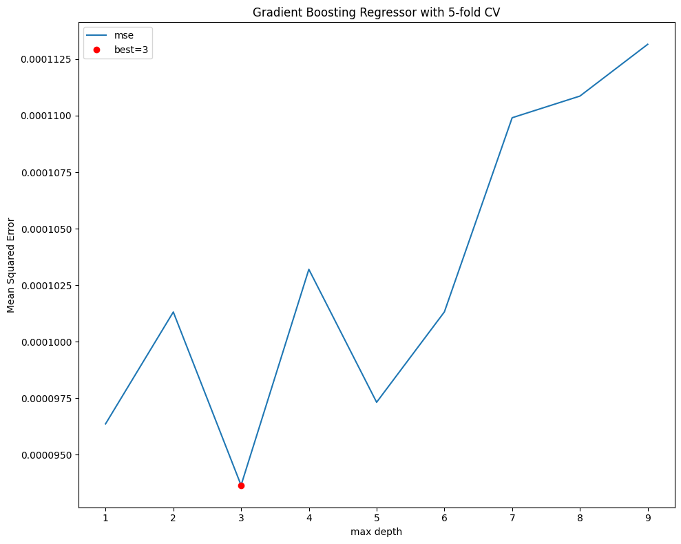
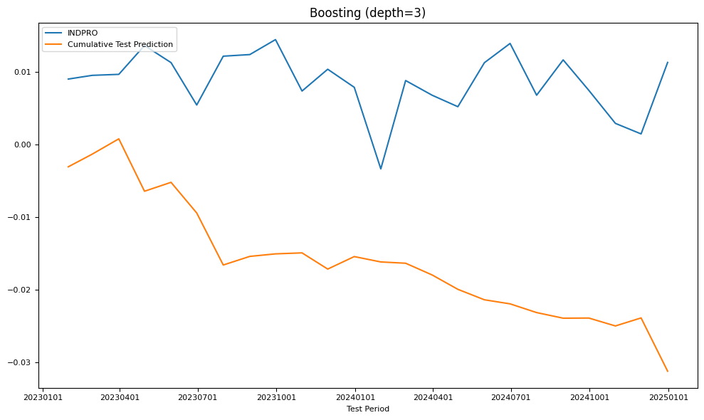
Gradient Boosting is an ensemble learning technique that builds models sequentially, where each new model corrects the errors of the previous ones. It uses decision trees as weak learners and minimizes the loss function by optimizing the model in the direction of the gradient of the loss. Key parameters include n_estimators (number of trees), learning_rate (step size for updates, controlling how much each tree contributes), and max_depth (tree depth, preventing overfitting). Gradient Boosting can be computationally expensive and prone to overfitting if not regularized using techniques like early stopping or shrinkage (learning_rate tuning).

from sklearn.ensemble import GradientBoostingRegressor
X_train, X_test, Y_train, Y_test = ts_split(X, Y)
scale = StandardScaler().fit(X_train)
X_train = scale.transform(X_train)
X_test = scale.transform(X_test)

# tune max_depth with 5-fold CV
n_splits=5
kf = KFold(n_splits=n_splits, shuffle=True, random_state=0)
mse = Series(dtype=float)
for i in range(1, 10): # tune max_depth for best performance
    boosted = GradientBoostingRegressor(max_depth=i, random_state=0)
    score = cross_val_score(boosted,
                            X_train,
                            Y_train,
                            cv=kf,
                            n_jobs=5,
                            verbose=VERBOSE,
                            scoring='neg_mean_squared_error').mean()
    mse.loc[i] = -score

fig, ax = plt.subplots(figsize=(10, 8))
mse.plot(ax=ax, ylabel='Mean Squared Error', xlabel='max depth',
         title=f"Gradient Boosting Regressor with {n_splits}-fold CV")
best = mse.index[mse.argmin()]
ax.plot(best, mse.loc[best], "or")
ax.legend(['mse', f"best={best}"])
plt.tight_layout()

# evaluate train and test MSE
name = f"Boosting (depth={best})"
model = GradientBoostingRegressor(max_depth=best,
                                  random_state=0).fit(X_train, Y_train)

Y_pred = Series(index=Y_test.index,
                data=model.predict(X_test).reshape((-1,)))
test[name] = mean_squared_error(Y_test, Y_pred)
train[name] = mean_squared_error(Y_train, model.predict(X_train))
final_models[name] = model

fig, ax = plt.subplots(figsize=(10, 6))
plot_date(pd.concat([Y_test.cumsum(), Y_pred.cumsum()], axis=1),
          legend1=[target_id, 'Cumulative Test Prediction'],
          title=name,
          xlabel='Test Period',
          fontsize=8,
          ax=ax)
plt.tight_layout()

DataFrame({'name': name,
           'train': np.sqrt(train[name]),
           'test': np.sqrt(test[name])}, index=['RMSE'])

	name	train	test
RMSE	Boosting (depth=3)	0.002704	0.007407

Feature importances:

# Show feature importance
top_n = 10
imp = Series(model.feature_importances_, index=X.columns).sort_values()
print(f"Gradient Boosting: Top {top_n} Feature Importances")
DataFrame.from_dict({i+1: {'importance': imp[s],
                           'series_id': s.split('_')[0],
                           'lags': s.split('_')[1],
                           'description': alf.header(s.split('_')[0])}
                     for i, s in enumerate(np.flip(imp.index[-top_n:]))},
                    orient='index')

Gradient Boosting: Top 10 Feature Importances

	importance	series_id	lags	description
1	0.140886	BUSLOANS	1	Commercial and Industrial Loans, All Commercia...
2	0.136621	CLAIMS	1	Initial Claims
3	0.031817	UEMPLT5	3	Number Unemployed for Less Than 5 Weeks
4	0.030436	M2REAL	3	Real M2 Money Stock
5	0.029806	USGOOD	1	All Employees, Goods-Producing
6	0.027816	M2SL	1	M2
7	0.022606	IPNMAT	1	Industrial Production: Nondurable Goods Materials
8	0.020286	DMANEMP	1	All Employees, Durable Goods
9	0.019784	EXCAUS	1	Canadian Dollars to U.S. Dollar Spot Exchange ...
10	0.018134	UNRATE	1	Unemployment Rate

Random Forest

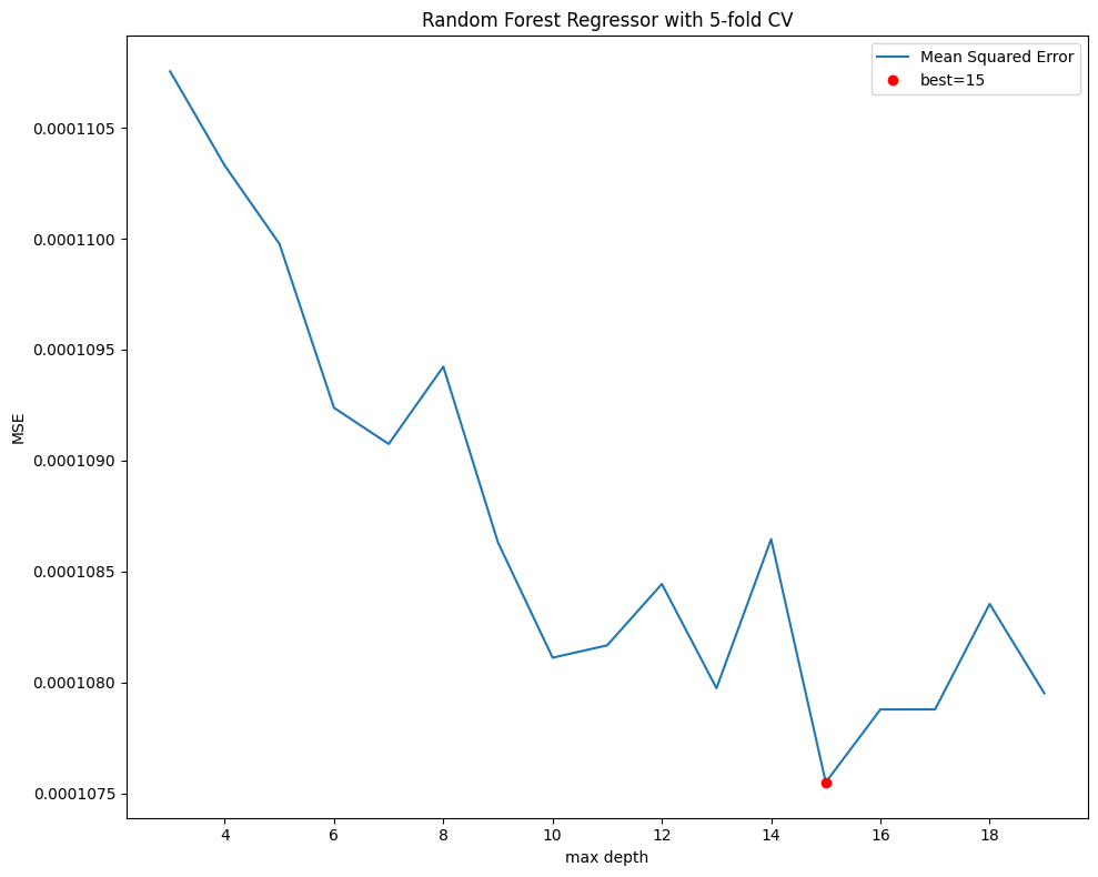
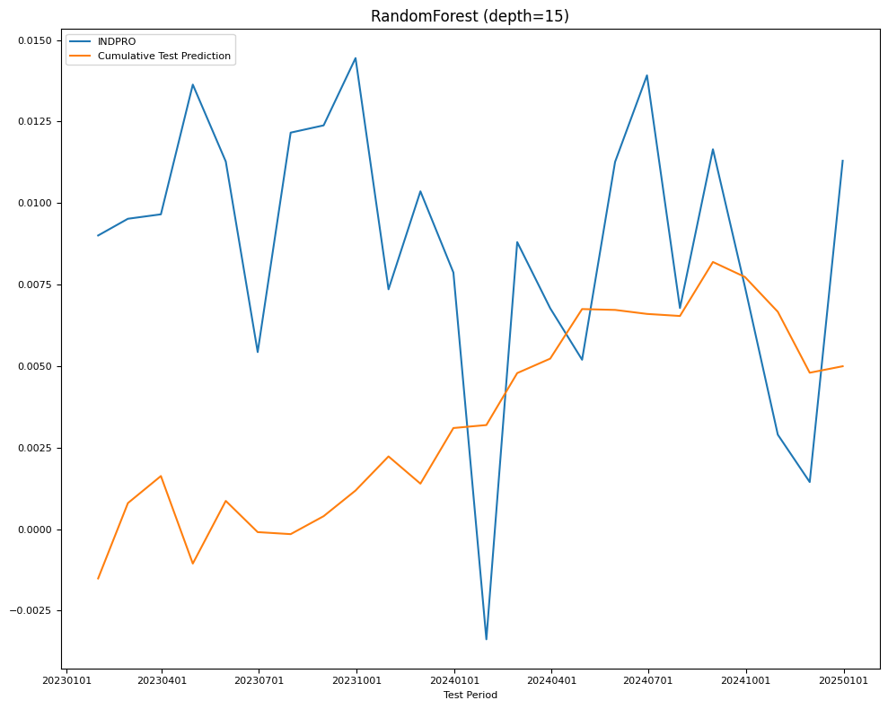
Random Forest is an ensemble learning method that builds multiple decision trees and combines their predictions to improve accuracy and reduce overfitting. It operates by randomly selecting subsets of the training data and features (using bootstrap sampling and feature bagging) to create diverse trees. The final prediction is determined by majority voting (for classification) or averaging (for regression). Key parameters include n_estimators (number of trees), max_depth** (maximum depth of each tree), max_features (number of features considered for splitting), and min_samples_split (minimum samples needed to split a node). Feature importance scores can be extracted to interpret which variables influence predictions most. Random Forest handles missing data well and mitigates overfitting through averaging multiple models.

from sklearn.ensemble import RandomForestRegressor
X_train, X_test, Y_train, Y_test = ts_split(X, Y)

# tune max_depth with 5-fold CV
n_splits=5
kf = KFold(n_splits=n_splits,
           shuffle=True,
           random_state=0)
mse = Series(dtype=float)
for i in range(3, 20): #tune for best performance
    model = RandomForestRegressor(max_depth=i, random_state=0)
    score = cross_val_score(model,
                            X_train,
                            Y_train,
                            cv=kf,
                            n_jobs=5,
                            verbose=VERBOSE,
                            scoring='neg_mean_squared_error').mean()
    mse.loc[i] = -score
    #print(i, np.sqrt(abs(score)))

fig, ax = plt.subplots(figsize=(10, 8))
mse.plot(ax=ax, ylabel='MSE', xlabel='max depth',
         title=f"Random Forest Regressor with {n_splits}-fold CV")
best = mse.index[mse.argmin()]
ax.plot(best, mse.loc[best], "or")
ax.legend(['Mean Squared Error', f"best={best}"])
plt.tight_layout()

name = f"RandomForest (depth={best})"
model = RandomForestRegressor(max_depth=best,
                              random_state=0).fit(X_train, Y_train)

Y_pred = Series(index=Y_test.index,
                data=model.predict(X_test).reshape((-1,)))
test[name] = mean_squared_error(Y_test, Y_pred)
train[name] = mean_squared_error(Y_train, model.predict(X_train))
final_models[name] = model

fig, ax = plt.subplots(figsize=(10, 8))
plot_date(pd.concat([Y_test.cumsum(), Y_pred.cumsum()], axis=1),
          legend1=[target_id, 'Cumulative Test Prediction'],
          title=name,
          xlabel='Test Period',
          fontsize=8,
          ax=ax)
plt.tight_layout()

DataFrame({'name': name,
           'train': np.sqrt(train[name]),
           'test': np.sqrt(test[name])}, index=['RMSE'])

	name	train	test
RMSE	RandomForest (depth=15)	0.00376	0.005875

Feature importance scores:

# Feature importance
top_n = 10
imp = Series(model.feature_importances_, index=X.columns).sort_values()
print(f"Random Forest: Top {top_n} Feature Importances")
DataFrame.from_dict({i+1: {'importance': imp[s],
                          'series_id': s.split('_')[0],
                          'lags': s.split('_')[1],
                          'description': alf.header(s.split('_')[0])}
                    for i, s in enumerate(np.flip(imp.index[-top_n:]))},
                   orient='index')

Random Forest: Top 10 Feature Importances

	importance	series_id	lags	description
1	0.051226	CLAIMS	1	Initial Claims
2	0.046733	BUSLOANS	1	Commercial and Industrial Loans, All Commercia...
3	0.044055	M2SL	1	M2
4	0.015825	USGOOD	1	All Employees, Goods-Producing
5	0.015268	UNRATE	1	Unemployment Rate
6	0.014617	UEMPLT5	3	Number Unemployed for Less Than 5 Weeks
7	0.014576	IPCONGD	1	Industrial Production: Consumer Goods
8	0.014529	UEMPLT5	1	Number Unemployed for Less Than 5 Weeks
9	0.014496	M1SL	1	M1
10	0.013855	DMANEMP	1	All Employees, Durable Goods

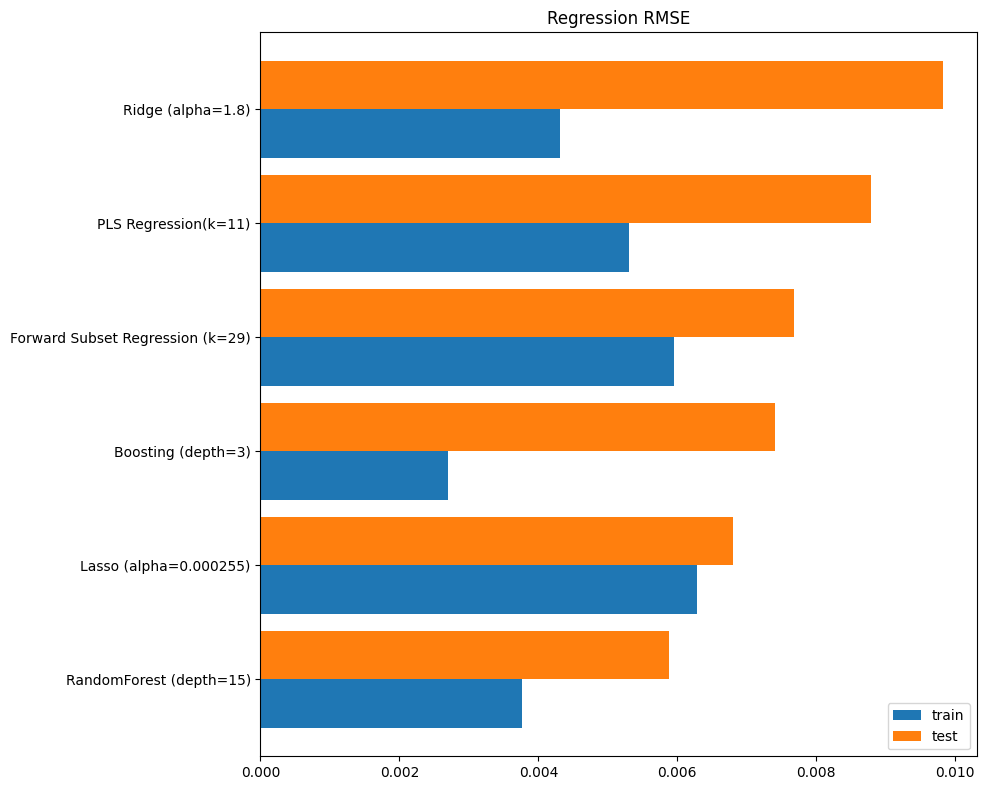
Summary:

The root mean squared error (RMSE) performance of all the models, based on train and test samples, is summarized in the following chart:

fig, ax = plt.subplots(figsize=(10, 8))
pd.concat([np.sqrt(r.to_frame()) for r in [train, test]], axis=1)\
  .sort_values('test')\
  .plot.barh(ax=ax, width=0.85)
ax.yaxis.set_tick_params(labelsize=10)
ax.set_title('Regression RMSE')
ax.figure.subplots_adjust(left=0.35)
plt.tight_layout()

References:

Gareth James, Daniela Witten, Trevor Hastie, Robert Tibshirani. “An Introduction to Statistical Learning with Applications in R”. New York, Springer, 2013.