Event Study

All strange and terrible events are welcome, but comforts we despise - Cleopatra

Event studies are a fundamental tool in financial research used to assess how specific events impact stock returns, see Mackinlay (1997). These events, such as mergers, earnings announcements, or regulatory changes, can cause deviations in stock prices known as abnormal returns. By comparing stock returns to a market benchmark, event studies help analysts determine whether an event had a statistically significant impact on a company’s stock price.

This notebook explores key methodologies used in event studies, including the computation of abnormal returns, cumulative abnormal returns, and buy-and-hold abnormal returns. Additionally, it delves into the announcement effect, which examines how stock prices react immediately around an event, and investigates potential pre- and post-announcement drifts. To account for overlapping event windows and cross-sectional dependencies, we apply statistical corrections based on the work of Kolari et al. (2010, 2018).

We also introduce frequency domain methods, leveraging the Fourier Transform and Convolution Theorem to efficiently compute cross-correlations between time series. Finally, we address the multiple testing problem, ensuring that statistical inferences remain valid when analyzing a large number of events.

import numpy as np
import pandas as pd
from pandas import DataFrame, Series
import matplotlib.pyplot as plt
from scipy.stats import norm
from statsmodels.stats.multitest import multipletests
from tqdm import tqdm
import warnings
from finds.database import SQL, RedisDB
from finds.structured import BusDay, Benchmarks, Stocks, CRSP, PSTAT
from secret import credentials, paths, CRSP_DATE
VERBOSE = 0
if not VERBOSE:
    warnings.simplefilter(action='ignore', category=FutureWarning)
#%matplotlib qt

# open connections
sql = SQL(**credentials['sql'], verbose=VERBOSE)
user = SQL(**credentials['user'], verbose=VERBOSE)
bd = BusDay(sql)
rdb = RedisDB(**credentials['redis'])
keydev = PSTAT(sql, bd, verbose=VERBOSE)
crsp = CRSP(sql, bd, rdb=rdb, verbose=VERBOSE)
bench = Benchmarks(sql, bd, verbose=VERBOSE)
imgdir = paths['images'] / 'events'

Abnormal returns

Event studies analyze how stock returns respond to specific company events, such as mergers or public announcements. These studies examine deviations from expected returns, known as abnormal returns, in the days surrounding the news release.

Let the event date be \(t = 0\), and define the stock return for firm \(i\) at time \(t\) as \(R_{i,t}\). To provide a benchmark, we also compute the returns of a relevant market or sector index, denoted \(R_{m,t}\). Then:

• Abnormal returns (AR): The deviation of a stock’s return from the market return: $\( AR_{i,t} = R_{i,t} - R_{m,t}\)$

• Average abnormal returns (AAR): The mean abnormal return across all firms: $\( AAR_t = \dfrac{1}{N} \sum_i^N AR_{i,t} \)$

• Cumulative average abnormal returns (CAR): The sum of average abnormal returns over time: $\( CAR_T = \sum_t AAR_t \)$

• Buy-and-hold average abnormal returns (BHAR): The average buy-and-hold abnormal returns across firms: $\( BHAR_T = \dfrac{1}{N} \sum_i^N \left[ \prod_t (1+ AR_{i,t}) - \prod_t (1+ R_{m,t}) \right] \)$

Announcement effect

The announcement effect refers to the immediate stock price movement around a news release. The nature of this reaction varies:

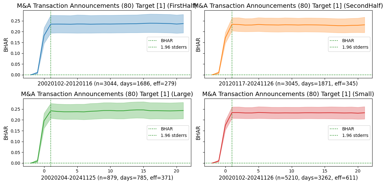
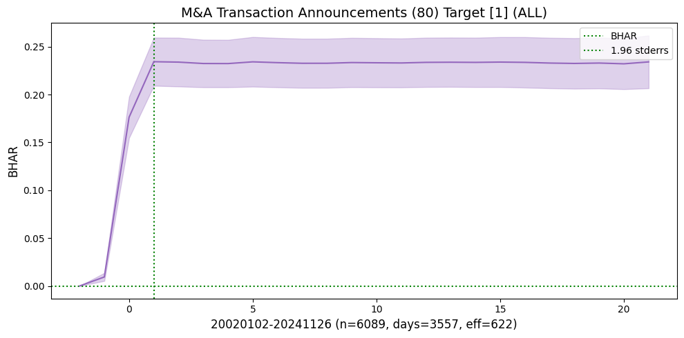
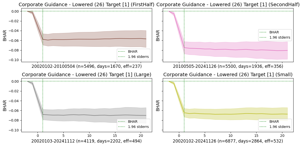
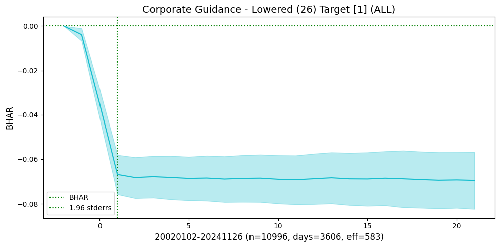
• An efficient reaction occurs when the stock price stabilizes at its new level after the event.

• An under-reaction happens when the price continues trending in the same direction post-announcement.

• An over-reaction is when the price initially spikes but then reverses course.

In historical data, pinpointing the exact announcement time can be challenging. To account for this uncertainty, studies often consider an announcement window, typically covering one day before and after the event.

• A pre-announcement drift may indicate information leakage before the official announcement.

• A post-announcement drift may suggest that investors either under- or over-reacted to the news.

When analyzing multiple events, researchers often aggregate returns for stocks with the same announcement date. However, Kolari et al. (2010) caution that even small correlations among abnormal returns can lead to significant over-rejection of the null hypothesis of zero abnormal returns. To correct for this cross-sectional dependence, the unbiased estimate of abnormal return variance is:

\[ \sigma^{2} = \dfrac{s^2}{n} (1 + (n - 1) \hat{r}) \]

where:

• \(\hat{r}\) is the average sample cross-sectional correlation of residuals,

• \(s^2\) is the (biased) cross-sectional standard deviation of abnormal returns.

In the next subsection, we explore how cross-correlations can be be measured efficiently using the Fourier Transform technique from the field of signal processing.

FinDS eventstudy module

The eventstudy module in the FinDS package provides a comprehensive tool for analyzing announcement effects.

from finds.backtesting import EventStudy
eventstudy = EventStudy(user, bench=bench, stocks=crsp, max_date=CRSP_DATE)

# event window parameters
left, right, post = -1, 1, 21
end = bd.offset(CRSP_DATE, left - post)
beg = 20020101
mindays = 1000

• Retrieve event dates and company roles from CapitalIQ Key Developments

# sorted list of all eventids and roleids, provided in keydev class
events = sorted(keydev.event.index)
roles = sorted(keydev.role.index)

# str formatter to pretty print descriptions, provided in keydev class
eventformat = lambda e, r: "{event} ({eventid}) {role} [{roleid}]"\
    .format(event=keydev.event[e], eventid=e, role=keydev.role[r], roleid=r) 

• Helper functions to retrieve size decile of universe stocks

class Universe:
    """Helper to lookup prevailing size decile of universe stocks"""
    def __init__(self, beg: int, end: int, stocks: Stocks, annual: bool = False):
        # whether to offset previous month or year end when lookup
        self.offset = stocks.bd.endyr if annual else stocks.bd.endmo
        
        # populate dictionary, keyed by permno and date, with size decile
        self.decile = dict()
        date_range = stocks.bd.date_range(start=self.offset(beg, -1), end=end,
                                          freq=12 if annual else 'e')
        for date in date_range:
            univ = crsp.get_universe(date)
            for permno in univ.index:
                self.decile[(permno, date)] = univ.loc[permno, 'decile']

    def __getitem__(self, item):
        """Returns size decile, else 0 if not universe stock"""
        permno, date = item
        return self.decile.get((permno, self.offset(date, -1)), 0)
    
univ = Universe(beg=beg, end=end, stocks=crsp)

• Define the event study pipeline:

  1. retrieve announcement dates for the desired event and test period

  2. filter the universe

  3. retrieve announcement window daily stock returns, and compute event study metrics

# run event study after screening stock universe
def event_pipeline(eventstudy: EventStudy,
                   beg: int,
                   end: int,
                   eventid: int,
                   roleid: int,
                   left: int,
                   right: int,
                   post: int) -> DataFrame:
    """helper to screen stock universe, and merge keydev events and crsp daily"""

    # Retrieve announcement dates for this event
    df = keydev.get_linked(
        dataset='keydev',
        date_field='announcedate',
        fields=['keydevid',
                'keydeveventtypeid',
                'keydevtoobjectroletypeid'],
        where=(f"announcedate >= {beg} "
               f"  and announcedate <= {end}"
               f"  and keydeveventtypeid = {eventid} "
               f"  and keydevtoobjectroletypeid = {roleid}"))\
               .drop_duplicates(['permno', 'announcedate'])\
               .set_index(['permno', 'announcedate'], drop=False)

    # Require universe size decile
    df['size'] = [univ[row.permno, row.announcedate] for row in df.itertuples()]

    # Call eventstudy to compute daily abnormal returns, with named label
    rows = eventstudy(label=f"{eventid}_{roleid}",
                      df=df[df['size'].gt(0)],
                      left=left,
                      right=right,
                      post=post,
                      date_field='announcedate')
    return df.loc[rows.to_records(index=False).tolist()] # restrict successful rows

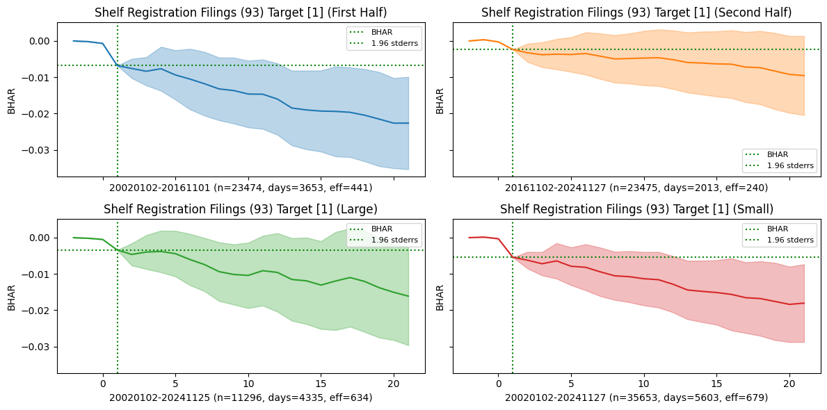
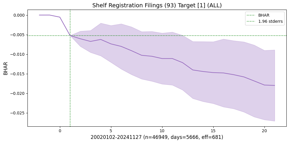
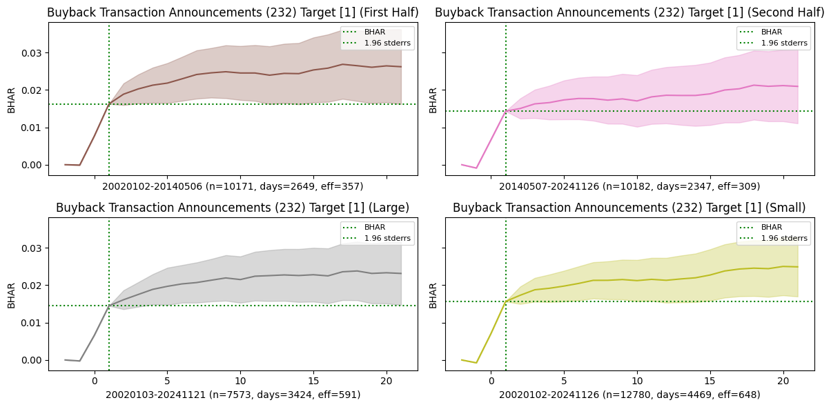
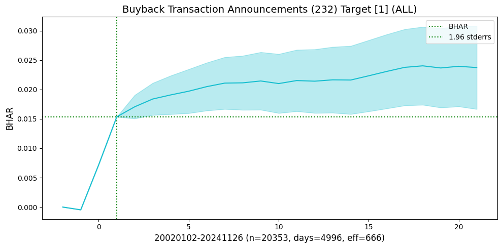
Examine and show subsample plots for events that exhibited large post-announcement drift

events_list = [[93, 1], [232, 1]]  # largest drift returns
for i, (eventid, roleid) in enumerate(events_list):
    df = event_pipeline(eventstudy,
                        eventid=eventid,
                        roleid=roleid,
                        beg=beg,
                        end=end,
                        left=left,
                        right=right,
                        post=post)
    halfperiod = np.median(df['announcedate'])
    sample = {'First Half': df['announcedate'].lt(halfperiod).values,
              'Second Half': df['announcedate'].ge(halfperiod).values,
              'Large': df['size'].le(5).values,
              'Small': df['size'].gt(5).values,
              'ALL': [],
             }
    fig, axes = plt.subplots(nrows=2, ncols=2, clear=True, figsize=(12, 6),
                             sharex=True, sharey=True)
    axes = axes.flatten()
    for ifig, (label, rows) in enumerate(sample.items()):
        if ifig >= len(axes):
            plt.show()
            fig, ax = plt.subplots(clear = True, figsize=(10, 5))
        else:
            ax = axes[ifig]
        bhar = eventstudy.fit(model='sbhar', rows=rows)
        eventstudy.plot(model='sbhar',
                        title=eventformat(eventid, roleid) + f" ({label})",
                        drift=True,
                        ax=ax,
                        fontsize=(8 if ifig < len(axes) else 10),
                        c=f"C{i*5+ifig}")
        plt.tight_layout()
        plt.savefig(imgdir / (label + f"{eventid}_{roleid}.jpg"))
    plt.show()

Examine and show subsample plots for events that exhibited large announcement window returns

events_list = [[80,1], [26,1]]  # largest announcement window returns
for i, (eventid, roleid) in enumerate(events_list):
    #eventid, roleid = 50, 1
    #eventid, roleid = 83, 1
    df = event_pipeline(eventstudy,
                        eventid=eventid,
                        roleid=roleid,
                        beg=beg,
                        end=end,
                        left=left,
                        right=right,
                        post=post)
    halfperiod = np.median(df['announcedate'])
    sample = {'FirstHalf': df['announcedate'].lt(halfperiod).values,
              'SecondHalf': df['announcedate'].ge(halfperiod).values,
              'Large': df['size'].le(5).values,
              'Small': df['size'].gt(5).values,
              'ALL': []}
    fig, axes = plt.subplots(nrows=2, ncols=2, clear=True, figsize=(12, 6),
                             sharex=True, sharey=True)
    axes = axes.flatten()
    for ifig, (label, rows) in enumerate(sample.items()):
        if ifig >= len(axes):
            plt.show()
            fig, ax = plt.subplots(clear = True, figsize=(10, 5))
        else:
            ax = axes[ifig]
        bhar = eventstudy.fit(model='sbhar', rows=rows)
        eventstudy.plot(model='sbhar',
                        title=eventformat(eventid, roleid) + f" ({label})",
                        drift=False,
                        ax=ax,
                        c=f"C{i*5+ifig}")
        plt.tight_layout()
        plt.savefig(imgdir / (label + f"{eventid}_{roleid}.jpg"))
    plt.show()

Fourier transforms

Cross-sectional Correlations

Kolari et al. (2018) address event windows that partially overlap in calendar time. To account for this overlap and cross-sectional correlation effects, they adjust the variance estimate as follows:

\[ \sigma^{2} = \dfrac{s^2}{n} m (1 + \tau (n - 1) \rho) \]

where:

• \( m \) = length of the event window,

• \( \tau \) = proportion of overlapping days between event windows,

• \( \rho \) = ratio of average covariance between abnormal returns to their variance.

If all events share the same calendar date, such that all event windows fully overlap, then \( \rho \) simplifies to the average cross-sectional correlation of residuals during the estimation period.

To estimate \( \rho \), we assume cross-sectional correlations arise mainly from time misalignment. By shifting and aligning event window residuals for each stock pair to maximize their correlation, we approximate \( \rho \) as the average of these best-aligned correlations. We leverage the methodology of Fourier transforms and convolutions to effeciently compute all pairs of correlations.

Fast Fourier Transforms

Fourier transforms allow us to express a time series (or any function) as a sum of sinusoids. Given a function over an interval of length ( L ), we can decompose it into sinusoidal components with periods ( L, L/2, L/3, ) etc. Each component has:

• A magnitude (scale factor)

• A phase (shift)

• A frequency (inverse of the period)

This means that any function can be represented as a weighted sum of sinusoidal waves. By using complex numbers, we can efficiently store and manipulate these sinusoidal components in Fourier space rather than the original time domain. The Fast Fourier Transform (FFT) is an efficient algorithm for computing the Discrete Fourier Transform (DFT). The DFT converts a sequence of time-domain data points into its sinusoidal coefficients, converting it from real space to frequency space. The Inverse Fast Fourier Transform reconstructs the original function.

Convolution Theorem

Convolution is a mathematical operation that combines two functions (\( f \) and \( g \)) to produce a third function (\( f * g \)), expressing how one function modifies the other:

\[ (f * g)(t) = \int_{-\infty}^{\infty} f(s) g(t - s) ds \]

In one dimension, convolution acts like a moving average, smoothing a time series by weighting neighboring values. In two dimensions, it applies filters (e.g., blurring, edge detection) in image processing.

In signal processing, frequency-domain techniques efficiently compute cross-correlations across various time shifts. Instead of directly computing correlations for every possible lag (which is computationally expensive), we leverage the Convolution Theorem. A key property of Fourier transforms is that convolution in the time domain corresponds to multiplication in the frequency domain.

\[ \mathcal{F}\{f(t) * g(t)\} = \mathcal{F}\{f(t)\} \mathcal{F}\{g(t)\} \]

Since direct convolution requires \(O(N^2)\) operations, computing it directly is slow. However:

1. We can first apply the Fast Fourier Transform (FFT) to convert both functions into frequency space in \(O(N \log N)\) time.

2. In frequency space, convolution is just element-wise multiplication of Fourier coefficients, which is very fast.

3. We then apply the Inverse FFT (IFFT) to obtain the final result in \(O(N \log N)\) time.

# best alignment and cross-correlation using convolution theorem method
from scipy.fft import rfft, irfft
def fft_align(X):
    """Find best alignment, max cross-correlation and indices of all pairs of columns"""

    def _normalize(X: np.ndarray) -> np.ndarray:
        """Helper to demean columns and divide by norm"""
        X = X - np.mean(X, axis=0)
        X = X / np.linalg.norm(X, axis=0)
        return X

    N, M = X.shape
    X = np.pad(_normalize(X), [(0, N), (0,0)])  # normalize and zero pad
    Y = rfft(np.flipud(X), axis=0)              # FFT of all series flipped
    X = rfft(X, axis=0)                         # FFT of all original series
    corr, disp, cols = [], [], []               # to accumulate results
    for col in range(M-1):  # at each iter: compute column col * all remaining columns
        conv = irfft(X[:, [col]] * Y[:, col+1:], axis=0)  # inverse of product of FFT
        corr.extend(np.max(conv, axis=0))
        shift = (N//2) + 1           # displacement location relative to center
        disp.extend(((np.argmax(conv, axis=0) + shift) % N) - shift + 1)
        cols.extend([(col, j) for j in range(col+1, M)])
    return corr, disp, cols

Z = np.random.uniform(size=(10000, 1))
fft_align(np.hstack((Z[:-1], Z[1:])))

([0.9998967076018761], [1], [(0, 1)])

#fft_align(np.hstack(np.hstack((Z[:-5], Z[5:])))[:,2:], Z[:-2]) 
fft_align(np.hstack((np.hstack((Z[:-5], Z[5:]))[:-2], Z[7:])))

([0.9997503757740265, 0.9993943885689067, 0.9996440440611477],
 [5, 7, 2],
 [(0, 1), (0, 2), (1, 2)])

Multiple testing

When testing a huge number of null hypotheses, we are bound to get some very testing small p-values by chance. Data snooping occurs when the analyst fits a great number of models to a dataset. When explanatory variables are selected using the data, t-ratios and F-ratios will be too large, thus overstating the importance of variables in the model. Multiple testing adjusts the hurdle for significance because some tests will appear significant by chance. The downside of doing this is that some truly significant strategies might be overlooked because they did not pass the more stringent hurdle. This is the classic tension between Type I errors and Type II errors. The Type I error is the false discovery (investing in an unprofitable trading strategy). The Type II error is missing a truly profitable trading strategy.

The Family-Wise Error Rate (FWER) controls the probability of making at least one false discovery. If all \( m \) null hypotheses are independent and true:

\[ \mathrm{FWER}(\alpha) = 1 - (1 - \alpha)^m \]

To maintain a stricter significance threshold, the Bonferroni correction divides the confidence level by the number of tests:

\[ \alpha' = \frac{\alpha}{m} \]

This ensures that across multiple tests, the probability of making even one false discovery remains below \( \alpha \). However, it can be overly conservative.

The false discovery rate (FDR) controls the proportion of false positives among rejected hypotheses. The Benjamini-Hochberg (BH) procedure is a widely used method for FDR control. Instead of adjusting individual significance thresholds like Bonferroni, BH ranks p-values and sets a significance cutoff where false discoveries remain within acceptable limits.

Compute BHAR and CAR of all events

restart_event = 0 # 75,1
for i, eventid in tqdm(enumerate(events), total=len(events)):
    if eventid <= restart_event:  # kludge to resume loop
        continue
    for roleid in roles:
        # retrieve all returns observations of this eventid, roleid
        df = event_pipeline(eventstudy,
                            beg=beg,
                            end=end,
                            eventid=eventid,
                            roleid=roleid,
                            left=left,
                            right=right,
                            post=post)
        if df['announcedate'].nunique() < mindays:  # require min number of dates
            continue

        # compute both BHAR and CAR averages, then plot and save
        bhar = eventstudy.fit(model='sbhar')
        car = eventstudy.fit(model='scar')
        #eventstudy.write()
        eventstudy.write_summary()
        #print(eventstudy.label, eventid, roleid)

        fig, axes = plt.subplots(1, 2, clear=True, figsize=(12, 4), num=1)
        eventstudy.plot(model='sbhar', ax=axes[0],
                        title=eventformat(eventid, roleid) + ' BHAR',
                        fontsize=8, vline=[right])
        eventstudy.plot(model='scar', ax=axes[1],
                        title=eventformat(eventid, roleid) + ' CAR',
                        fontsize=8, vline=[right])
        plt.tight_layout()
        plt.savefig(imgdir / f"{eventid}_{roleid}.jpg")

 45%|████▍     | 52/116 [20:04:50<22:46:35, 1281.17s/it]/home/terence/Dropbox/github/data-science-notebooks/finds/recipes/filters.py:28: RuntimeWarning: invalid value encountered in divide
  X = X / np.linalg.norm(X, axis=0)
 53%|█████▎    | 62/116 [23:27:18<18:41:48, 1246.45s/it]/home/terence/Dropbox/github/data-science-notebooks/finds/recipes/filters.py:28: RuntimeWarning: invalid value encountered in divide
  X = X / np.linalg.norm(X, axis=0)
 61%|██████    | 71/116 [26:38:56<16:18:29, 1304.66s/it]/home/terence/Dropbox/github/data-science-notebooks/finds/recipes/filters.py:28: RuntimeWarning: invalid value encountered in divide
  X = X / np.linalg.norm(X, axis=0)
100%|██████████| 116/116 [42:41:25<00:00, 1324.87s/it]  

Summarize BHAR’s of all events

# Create (eventid, roleid) multiindex for table of all BHAR's
df = eventstudy.read_summary(model='sbhar')\
               .set_index('label')\
               .drop(columns=['rho', 'tau', 'created'])
df = df[df['effective'] > 400].sort_values('post_t')  # sorted by post drift t-stat
multiIndex = DataFrame(df.index.str.split('_').to_list()).astype(int)
df.index = pd.MultiIndex.from_frame(multiIndex, names=['eventid', 'roleid'])
df['event'] = keydev.event[df.index.get_level_values(0)].values
df['role'] = keydev.role[df.index.get_level_values(1)].values
print("Post-Announcement Drift")
pd.set_option('display.max_rows', None)
df.set_index(['event', 'role']).drop(columns=['model'])

Post-Announcement Drift

		beg	end	rows	days	effective	window	window_t	post	post_t
event	role
Shelf Registration Filings	Target	20020102	20241127	46949	5666	681.0	-0.005224	-2.542320	-0.012755	-2.753130
Special/Extraordinary Shareholders Meeting	Target	20040106	20241127	6183	3353	534.0	-0.002029	-0.537886	-0.018210	-1.970180
Name Changes	Target	20020430	20241121	1563	1329	454.0	0.012626	1.944510	-0.023076	-1.968600
Changes in Company Bylaws/Rules	Target	20020430	20241127	27834	4825	592.0	-0.000070	-0.024033	-0.010242	-1.815650
Product-Related Announcements	Target	20020102	20241127	209897	5767	686.0	0.005712	4.608120	-0.004112	-1.607030
M&A Transaction Closings	Target	20020108	20241125	1508	1234	430.0	0.010726	1.184190	-0.019140	-1.506510
Auditor Changes	Target	20020103	20241127	9563	3888	609.0	-0.003402	-1.173250	-0.009535	-1.433420
Executive/Board Changes - Other	Target	20020101	20241127	222258	5766	685.0	-0.000533	-0.537347	-0.003171	-1.410500
Executive Changes - CFO	Target	20020102	20241127	22715	5544	677.0	-0.007618	-3.312440	-0.006563	-1.390520
Business Expansions	Target	20020102	20241127	58224	5709	688.0	0.002006	1.663570	-0.003755	-1.327890
Special Calls	Target	20030211	20241127	16738	4501	597.0	0.014764	1.100980	-0.014743	-1.257180
Executive Changes - CEO	Target	20020102	20241127	17079	5269	671.0	-0.005253	-1.572760	-0.007032	-1.120140
M&A Transaction Cancellations	Buyer	20020107	20241122	1508	1258	455.0	-0.000106	-0.019428	-0.010588	-1.037350
Client Announcements	Target	20020102	20241127	212795	5761	687.0	0.008237	7.380600	-0.002300	-0.908251
Follow-on Equity Offerings	Target	20020102	20241127	21917	5219	667.0	-0.030227	-5.005380	-0.007275	-0.892820
Investor Activism - Target Communication	Target	20020402	20241127	5248	3059	525.0	0.008690	2.362150	-0.004881	-0.801679
Earnings Calls	Target	20020108	20241127	236084	5442	654.0	0.000499	0.481335	-0.002042	-0.761636
Strategic Alliances	Target	20020102	20241127	29517	5463	679.0	0.010685	2.626260	-0.003538	-0.741016
Lawsuits & Legal Issues	Target	20020101	20241127	41158	5599	682.0	-0.000897	-0.413061	-0.002723	-0.677482
Investor Activism - Activist Communication	Target	20020102	20241126	8556	3875	576.0	0.014757	4.288130	-0.004063	-0.657731
Corporate Guidance - Lowered	Target	20020102	20241126	10996	3606	583.0	-0.066909	-14.887900	-0.002680	-0.590799
Private Placements	Buyer	20020103	20241127	11631	4362	645.0	0.000440	0.272817	-0.002208	-0.569800
M&A Transaction Announcements	Seller	20020101	20241127	12325	4804	662.0	0.009878	2.630630	-0.002869	-0.472392
M&A Transaction Closings	Buyer	20020101	20241127	43177	5699	687.0	0.004541	3.186290	-0.001394	-0.464066
Company Conference Presentations	Target	20041101	20241127	339716	4975	592.0	0.001272	1.292770	-0.001116	-0.455673
M&A Calls	Target	20031027	20241125	7218	3305	566.0	0.059589	8.955770	-0.002523	-0.436285
Index Constituent Adds	Target	20020102	20241127	29372	2248	517.0	-0.004618	-1.557500	-0.002675	-0.417274
Buyback Transaction Closings	Target	20020103	20241123	13012	3913	620.0	0.003593	1.725140	-0.001955	-0.416104
M&A Rumors and Discussions	Target	20020918	20241127	21747	4605	584.0	0.013315	4.876590	-0.001790	-0.409002
Shareholder/Analyst Calls	Target	20020108	20241127	24420	4417	585.0	0.001265	0.428922	-0.002059	-0.313663
Labor-related Announcements	Target	20020111	20241121	3975	2485	485.0	0.001723	0.546605	-0.002090	-0.306394
Business Reorganizations	Target	20020102	20241122	4398	2766	519.0	-0.001773	-0.381681	-0.002317	-0.301770
Conferences	Participant	20070125	20241127	296636	3676	451.0	-0.000775	-0.643617	-0.000928	-0.281036
M&A Transaction Announcements	Buyer	20020101	20241127	25352	5501	682.0	0.010533	3.253760	-0.001108	-0.268724
Delayed SEC Filings	Target	20020102	20241127	13297	2078	519.0	-0.017189	-3.797660	-0.001306	-0.113672
Earnings Release Date	Target	20020411	20241127	226653	5294	632.0	-0.000074	-0.071140	-0.000190	-0.069660
M&A Transaction Closings	Seller	20020101	20241127	18467	5138	672.0	0.003516	1.461850	-0.000303	-0.069015
M&A Transaction Announcements	Target	20020102	20241126	6089	3557	622.0	0.234380	18.265800	-0.000214	-0.028792
Discontinued Operations/Downsizings	Target	20020102	20241127	18782	4447	594.0	-0.009840	-2.844410	-0.000069	-0.010337
Fixed Income Offerings	Target	20020101	20241127	28237	5403	677.0	-0.004932	-2.922310	0.000168	0.047205
Corporate Guidance - New/Confirmed	Target	20020101	20241127	148835	5649	687.0	-0.001445	-0.883251	0.000366	0.133957
Private Placements	Target	20020103	20241127	15216	5057	657.0	0.023461	4.328510	0.002351	0.223887
Seeking Acquisitions/Investments	Target	20020103	20241125	37787	5239	668.0	-0.000697	-0.305334	0.001316	0.366793
Board Meeting	Target	20020204	20241120	6563	2705	473.0	0.002824	0.980749	0.002164	0.375795
Considering Multiple Strategic Alternatives	Target	20040324	20241122	4017	2491	479.0	-0.008435	-1.135750	0.012629	0.556299
Announcements of Sales/Trading Statement	Target	20020102	20241119	12367	3306	588.0	0.004235	1.329410	0.005084	0.662073
Debt Financing Related	Target	20020102	20241127	41158	5708	684.0	0.004347	2.013270	0.002883	0.696258
Annual General Meeting	Target	20020122	20241127	71528	5094	620.0	0.001460	0.950287	0.004452	0.760826
Seeking to Sell/Divest	Target	20020110	20241125	5250	2922	504.0	-0.002623	-0.531814	0.006912	0.809188
End of Lock-Up Period	Target	20020115	20241126	7107	3293	565.0	-0.060075	-9.088620	0.007541	1.033670
Buyback Tranche Update	Target	20020107	20241127	113233	5073	646.0	0.000906	0.559217	0.002991	1.077510
Announcements of Earnings	Target	20020101	20241127	343641	5712	685.0	0.000446	0.305990	0.002854	1.128810
Analyst/Investor Day	Target	20040204	20241126	6664	3353	548.0	0.008374	3.238440	0.006292	1.208400
Investor Activism - Proxy/Voting Related	Target	20020107	20241126	7449	3165	530.0	-0.001100	-0.472323	0.011292	1.211770
Delistings	Target	20020102	20241127	17906	4928	625.0	-0.020833	-3.871270	0.016593	1.223670
Impairments/Write Offs	Target	20020408	20241126	23529	3527	521.0	-0.003683	-1.122100	0.008273	1.460700
Corporate Guidance - Raised	Target	20020103	20241126	20044	4162	631.0	0.033832	11.737600	0.006226	1.547110
Index Constituent Drops	Target	20020107	20241126	18202	3039	507.0	-0.003266	-0.751127	0.017488	1.557680
Buyback - Change in Plan Terms	Target	20020102	20241126	6897	3412	605.0	0.009150	3.837660	0.008018	1.846240
Buyback Transaction Announcements	Target	20020102	20241126	20353	4996	666.0	0.015343	7.037260	0.008389	2.327460

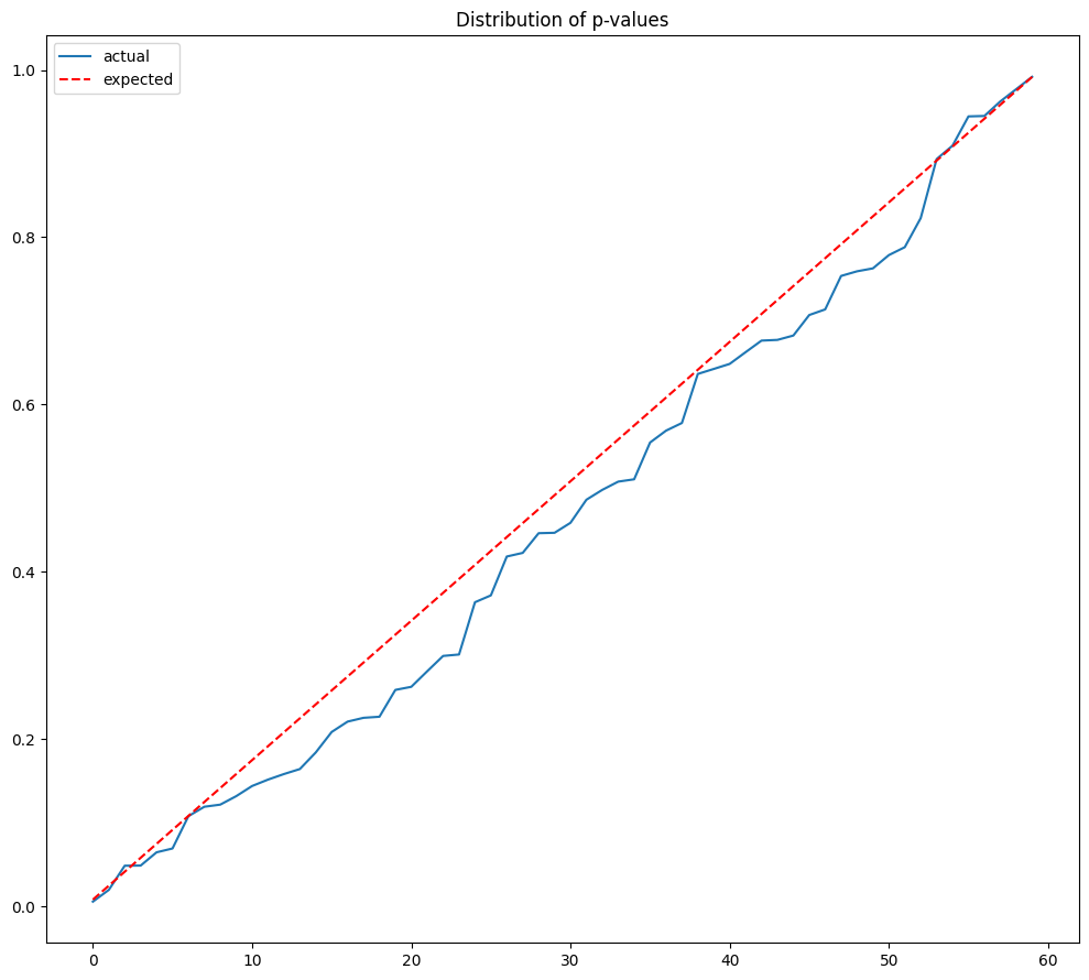
# Expected p-values (with continuity correction)
pvals = norm.cdf(-df['post_t'].abs()) * 2
fig, ax = plt.subplots(1, 1, clear=True, figsize=(10, 9))
ax.plot(sorted(pvals))
ax.plot([0, len(pvals)-1], [0.5/len(pvals), (len(pvals)-0.5)/len(pvals)], 'r--')
ax.set_title('Distribution of p-values')
ax.legend(['actual', 'expected'])
plt.tight_layout()

# Number of rejections with uncorrected pvals
#argmin = np.argmin(pvals)
#header = df.iloc[argmin][['event', 'role', 'days', 'effective', 'post_t']]
alpha = 0.05
uncorrected = DataFrame({'rejections': sum(pvals < alpha),
                         'min p-value': min(pvals)},
                        index=['uncorrected'])
uncorrected.round(4)

	rejections	min p-value
uncorrected	4	0.0059

Bonferroni correction

The best-known FWER test is called the Bonferroni test which adjusts for the multiple tests. Given the chance that one test could randomly show up as significant, the Bonferroni requires the confidence level to increase. Instead of 5%, you take the 5% and divide by the number of tests, that is, 5%/10 = 0.5%. Again equivalently, you need to be 99.5% confident with 10 tests that you are not making a single false discovery. In terms of the t-statistic, the Bonferroni requires a statistic of at least 2.8 for 10 tests. For 1,000 tests, the statistic must exceed 4.1.

It sets the threshold for rejecting each hypothesis to \(\alpha/m\), by applying the union bound inequality:

\[\mathrm{FWER}(\alpha) = \mathrm{Pr}(\cup_{j=1}^{m} A_j) \le \sum_{j=1}^{m} \mathrm{Pr}(A_j) \le m \times \frac{\alpha}{m} = \alpha\]

where \(A_j\) denotes the probability of rejecting the \(j\)-th hypothesis. The Bonferroni correction can be quite conservative, in the sense that the true FWER is often quite a bit lower than the nominal (or target) FWER;

# The Bonferroni p-values bonf are simply the uncorrected pvalues multiplied by
# the number of samples and truncated to be less than or equal to 1.  
reject, bonf_corrected, _, _ =  multipletests(pvals, alpha=alpha, method='bonferroni')
bonf = DataFrame({'rejections': np.sum(bonf_corrected < alpha),
                  'min p-value': np.min(bonf_corrected)},
                 index=['bonferroni'])
pd.concat([uncorrected, bonf], axis=0).round(4)

	rejections	min p-value
uncorrected	4	0.0059
bonferroni	0	0.3542

Holm’s step-down procedure

Holm’s method, also known as Holm’s step-down procedure or the Holm-Bonferroni method, is an alternative to the Bonferroni procedure. Holm’s method method controls the FWER, but it is less conservative than Bonferroni, in the sense that it will reject more null hypotheses, typically resulting in fewer Type II errors and hence greater power. Holm’s method makes no independence assumptions about the hypothesis tests, and is uniformly more powerful than the Bonferroni method – it will always reject at least as many null hypotheses as Bonferroni– and so it should always be preferred. It is worth noting that in Holm’s procedure, the threshold that we use to reject each null hypothesis actually depends on the values of all the p-values.

The Holm method begins by sorting the tests from the lowest p-value (most significant) to the highest (least significant), and comparing a threshold computed with the Holm function. In contrast to the Bonferroni, which has a single threshold for all tests, the other tests will have a different hurdle under Holm. Starting from the first test, we sequentially compare the p-values with their hurdles. When we first come across the test such that its p-value fails to meet the hurdle, we reject this test and all others with higher p-values.

# Holm method
reject, holm_corrected, _, _ =  multipletests(pvals, alpha=alpha, method='holm')
holm = DataFrame({'rejections': np.sum(holm_corrected < alpha),
                  'min p-value': np.min(holm_corrected)},
                 index=['holm'])
pd.concat([uncorrected, bonf, holm], axis=0).round(4)

	rejections	min p-value
uncorrected	4	0.0059
bonferroni	0	0.3542
holm	0	0.3542

Benjamin-Hochberg procedure

The false discovery rate approach allows an expected proportional error rate. As such, it is less stringent than both the Bonferroni and the Holm test. FDR control is much milder – and more powerful – than FWER control, in the sense that it allows us to reject many more null hypotheses, with a cost of substantially more false positives.

Similar to the Holm test, Benjamin-Hochberg also relies on the distribution of test statistics. However, in contrast to the Holm test that begins with the most significant test, the Benjamin-Hochberg approach starts with the least significant. We sort the tests from the lowest p-value (most significant) to the highest (least significant). Starting from the last test, we sequentially compare the p-values with their Benjamin-Hochberg thresholds. When we first come across the test such that its p-value falls below its threshold, we declare this test significant and all tests that have a lower p-value.

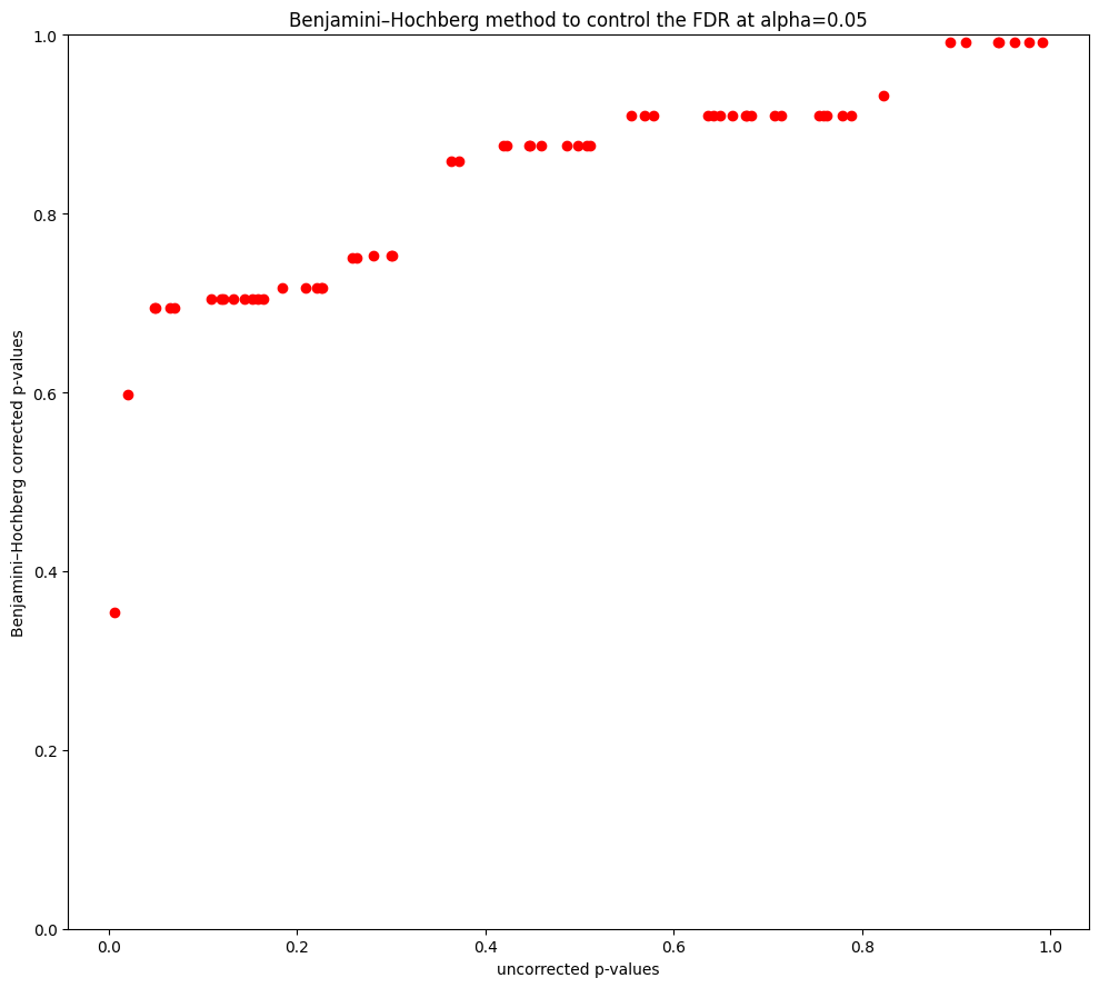
The multipletests function can be used to carry out the Benjamini–Hochberg procedure. The q-values output by the Benjamini–Hochberg procedure can be interpreted as the smallest FDR threshold at which we would reject a particular null hypothesis. For instance, a q-value of 0.1 indicates that we can reject the corresponding null hypothesis at an FDR of 10% or greater, but that we cannot reject the null hypothesis at an FDR below 10%.

# Benjamini-Hochberg method
reject, fdr_bh_corrected, _, _ =  multipletests(pvals, alpha=alpha, method='fdr_bh')
fdr_bh = DataFrame({'rejections': np.sum(fdr_bh_corrected < alpha),
                    'min p-value': np.min(fdr_bh_corrected)},
                   index=['fdr_bh'])
pd.concat([uncorrected, bonf, holm, fdr_bh], axis=0).round(4)

	rejections	min p-value
uncorrected	4	0.0059
bonferroni	0	0.3542
holm	0	0.3542
fdr_bh	0	0.3542

# Plot uncorrected and corrected p-values from Benjamini-Hochberg method
fig, ax = plt.subplots(figsize=(10, 9))
ax.scatter(pvals, fdr_bh_corrected, color='red')
ax.set_ylim(bottom=0, top=1)
ax.set_title(f"Benjamini–Hochberg method to control the FDR at alpha={alpha}")
ax.set_xlabel('uncorrected p-values')
ax.set_ylabel('Benjamini–Hochberg corrected p-values')
plt.tight_layout()

References

Kolari, James W. and Pynnonen, Seppo, 2010, “Event Study Testing with Cross-sectional Correlation of Abnormal Returns”. The Review of Financial Studies, 23(11), 3996-4025

Kolari, James W., Paper, Bernd, and Pynnonen, Seppo, 2018, “Event Study Testing with Cross-sectional Correlation Due to Partially Overlapping Event Windows”, working paper

MacKinlay, A. Craig “Event Studies in Economics and Finance”, Journal of Economic Literature, March 1997.

MIT License. Copyright 2021-2025 Terence Lim